The Memory Wall.
Download the PDF 48 pages · 3.2 MB
Get the result on a box you own, without data-centre memory. Claim the job, not the model.
Final Draft, written 11th November 2026. Figures are dated snapshots, last checked 9 November 2026. The argument rests on the ratios in section 14, not on any single figure.
Executive summary
Why does everyone need so many data centres? And if Europe wants its AI on its own soil, what does it do instead?
The short answer to the first question is memory. Every word a model writes means reading the model, and the whole conversation so far, back out of memory. The chip spends most of its time waiting for that read. One person chatting barely notices. An agent in production does: it re-reads a short book of context to write one line, and a business runs a great many agents at once. Each one keeps its own notes on its conversation, and those notes are never shared. Agents in production are a memory problem, not a maths problem.
The industry’s answer is to buy the memory: in GPUs by the hundred, in whole wafers, in buildings by the gigawatt. That is why the data centres keep coming. Britain cannot take that answer. In 2026 its grid operator expected to connect about 5 GW of data centres by 2030, with a queue of about 73 GW behind it. A firm that needs the capacity this year is not getting it from a queue.
So this paper takes the other road. It holds the memory fixed and changes the work to fit it.
It runs in three acts. Act one sets out what agents in production need, and why the old fix of moving memory closer stops working on a box you own. Act two takes eight ways the industry cuts memory, all real and all deployed, and finds where each one breaks on that box. Most break at the same point: more than one agent at once. Act three is the alternative. Small models are sized to the job and held whole in memory, each kind of agent is routed to the model it needs, and the box does not grow.
The claim, put plainly so it can be attacked: get the result on a box you own, without data-centre memory. Claim the job, not the model. I am not claiming frontier capability in a server room. I am claiming the finished piece of work, and for most of what a business wants automated, that is what it was paying for.
It does not claim that the box beats a batched data centre per answer. It does not. Nor that cloud costs more to start, or that smaller is cheaper per token. What the box wins is the right to own the thing at all, on data that never leaves the building.
How to read this paper
This paper was written with the non-technical human reader in mind. I have broken this problem down as simply as possible. My challenge to you as the reader is to read as far as you can without throwing the file through ChatGPT to summarise it.
Every claim carries its evidence class in the sentence that makes it: measured, derived, a position, or my reasoning. Figures are dated snapshots, last checked 9 November 2026. The argument rests on the ratios in section 14, not on any single figure.
The diagrams are there to help you picture what the text is saying. They are not extra evidence. Every number in a diagram comes from the text and its references, and where a diagram shows a pattern rather than a measurement, or adds arithmetic of my own, its caption says so. There are twenty-one, numbered in the order they appear.
The wall behind this thesis is about thirty years old. What is new is that its symptoms are starting to reach people who have never heard of it: dearer memory, dearer laptops, more data centres. I expect more in the coming months, and that is a bet, not a finding. When they reach the news, this paper should help you recognise them and understand the cause. Use that for your own business, or simply to be the person who can explain it at a dinner party. It starts with a quick physics reminder and builds up from there.
Physics and scale: a quick reminder
For most readers it’s probably been years since your last physics lesson at school, so here’s a quick reminder. Three ideas carry this paper: energy, power and scale.
Energy is something we use every day and rarely think about. Most of us only meet it on a food label, as calories. One kilocalorie is about 4,200 joules, the energy needed to warm one kilogram of water by one degree Celsius. An adult is advised to eat about 2,000 kcal a day. Spread across the day, that keeps a person running at about 100 watts, and the brain takes a fifth of it.
This paper is about electrical energy, and the unit most people know there is the one on their bill, the kilowatt-hour (kWh): one kilowatt drawn for one hour, or 3.6 million joules. At 2026 prices a unit costs about 25p. Electricity is cheap. As the rest of this paper shows, the bill that binds is memory.
Joules, kilocalories and kilowatt-hours all measure the same thing, energy as an amount, and none of them is easy to picture. So this paper uses one unit you can: the cup of coffee. Boiling the water for one cup takes about 84,000 joules. On a food label that would read as about 20 kcal. On your bill it is about 0.023 kWh, roughly half a penny. Turn it round and one kilowatt-hour would boil about 43 cups. (As an English writer, I’m surprised it isn’t cups of tea. The kettle doesn’t know the difference.) A cup measures energy, not water. Data centres use water too, but that is a different sum and a different paper. From here on, one unit: the cup.
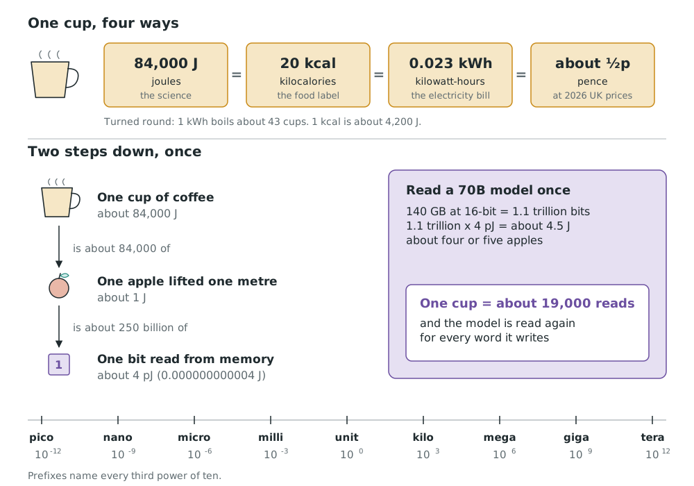
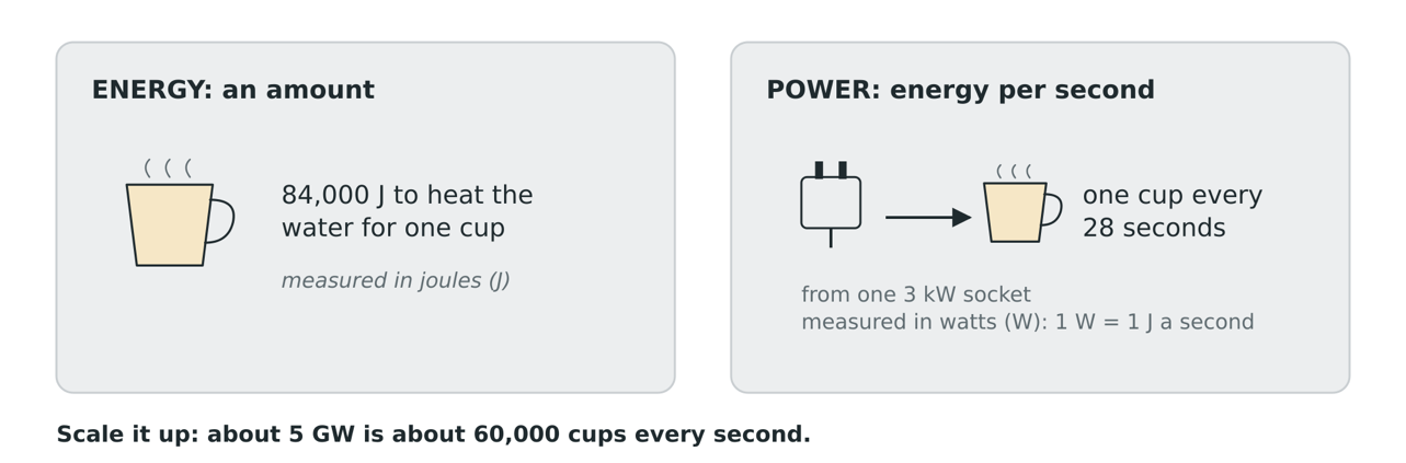
Power is how fast energy is spent: energy per second. One watt is one joule a second, so read watts as cups per second. A British kettle draws about 3 kW, the whole of one socket, and boils a cup in under half a minute. A gigawatt is a thousand million joules every second, which is a gigajoule, about 12,000 cups, every second (Figure 2).
Scale is the idea that makes the other two readable.
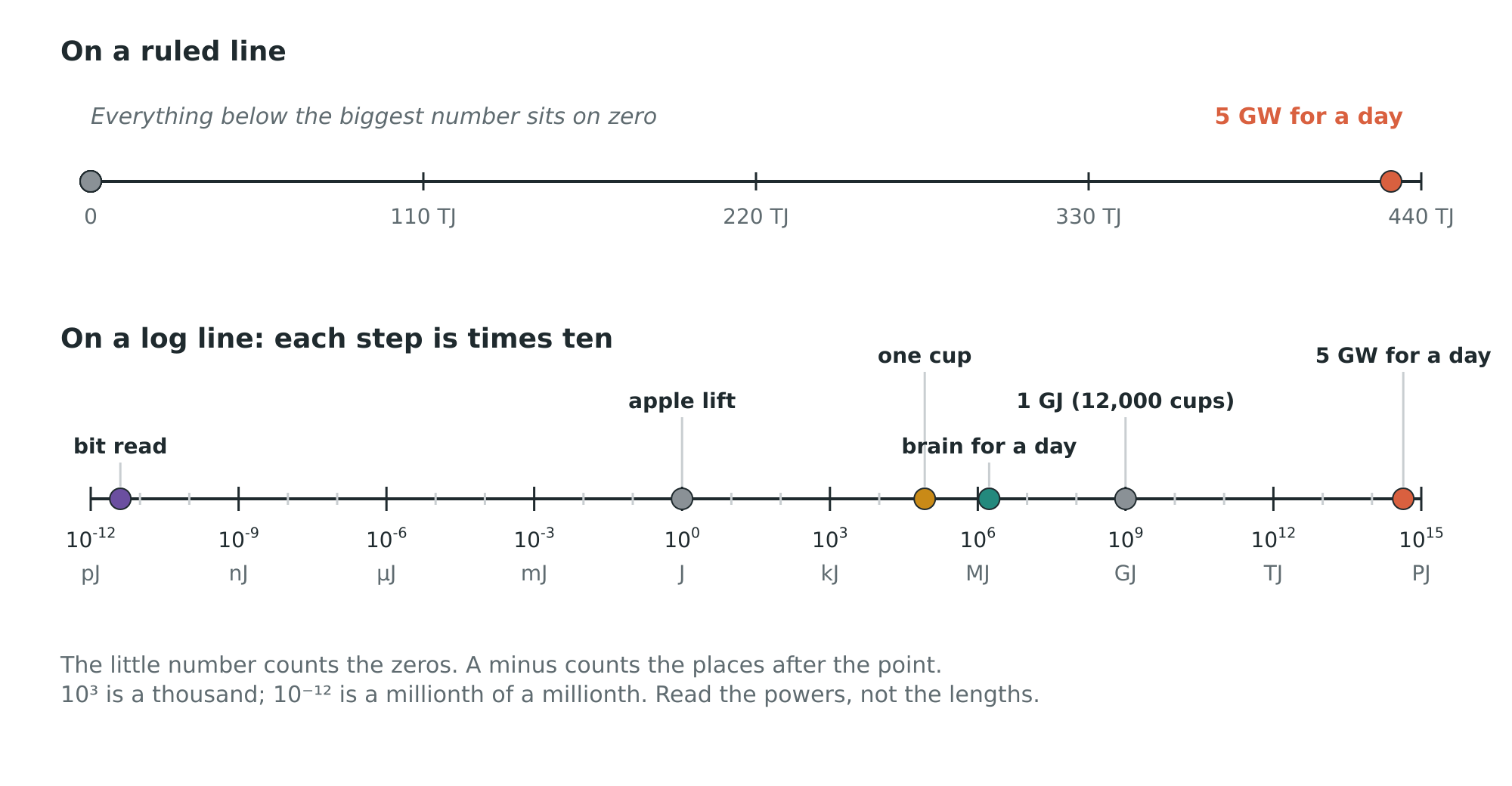
The numbers in this paper run from a few picojoules to hundreds of terajoules, about twenty-six powers of ten. No ordinary chart can hold that. Put them on a ruled line and everything but the largest sits on top of zero.
So the diagrams use a logarithmic scale, written in powers of ten. On a log scale each step is not plus one but times ten. 103 is a thousand, 106 is a million, and 10-12 is a millionth of a millionth. The little number counts the zeros, and a minus sign counts the places after the decimal point. The prefixes are only names for every third step: milli is 10-3, kilo 103, giga 109. That is how a picojoule and a gigajoule fit on one line.
One warning. A log scale makes big gaps look small. Two points one step apart look like neighbours, but one is ten times the other. On these diagrams, read the powers, not the lengths (Figure 3).
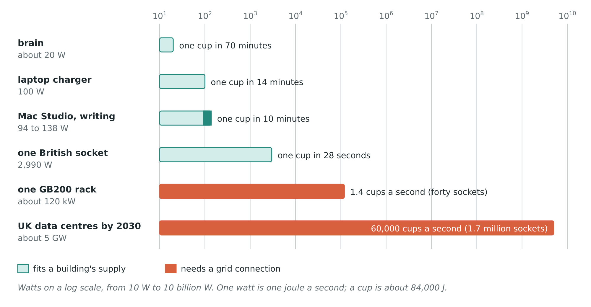
Here is power on that scale, from the brain to every data centre Britain expects to connect by 2030 (Figure 4).
Memory climbs the same ladder. Models are counted in gigabytes (109 bytes) and memory speed in terabytes a second (1012 bytes). They read and write in tokens of about three quarters of a word, and the gap between what an agent reads and what it writes is where this paper starts (Figure 5, in section 2).
Opening
Every leap in what we ask computers to do has hit a wall, and every wall has been answered by pulling a different lever. The first lever is scale: more power, more chips, more users sharing them. The second is more work from every watt, and since Apollo most of that has come from shrinking.
The room-sized machines that computed the flight to the Moon, five IBM System/360 Model 75s on the ground at Houston, became the phone in your pocket because the parts got smaller and closer together, so each step cost less and each trip the data made was shorter. That lever is now pressing on physics. Memory cells are packed so tightly that working one row hard enough can flip bits in the next, and moving memory any closer means stacking it beside the chip or holding the whole model on the chip itself, at a price only the biggest buyers pay. In the UK even the first lever is mostly out of reach. In 2026 Britain’s grid operator expected to connect about 5 GW of data centres by 2030. Behind that sat a queue of about 73 GW, perhaps half of it speculative. It does not matter which half. So I went looking for a third lever. The industry already squeezes its data, fewer bits per number and fewer numbers per word, yet it keeps asking for more of it in total. The third lever starts from the job and asks how little it needs. Not more power. Not a shorter trip. Less to carry.
Why less to carry? Because on a box you own, the trip is the bill. Every word a model writes means reading the model, and the whole conversation so far, back out of memory. That is the memory wall. Others have reached it from the chip side (Gholami et al. 2024; Singh 2026; Yuan and Long 2026). I reached it from agents on a box a business owns, and that route leads somewhere theirs does not: get the result on a box you own, and claim the job, not the model.
Thesis
Why does everyone need so many data centres? And if Europe wants its AI on its own soil, what does it do instead?
Thesis 2 priced the chip. It said that where a computation physically runs fixes what it costs and how long it takes, and I stand by it. But routing is a decision about compute, and compute is not the bill that binds. Route every token perfectly and there is a second bill underneath, and it is the one that decides whether you can run the thing at all. That bill is memory: how much of it the model has to hold, and how fast the chip can read it back.
I got here the way I got to Thesis 2, by following a bill I could not explain. At Keystone, my first company, I pushed an agent into production and the token costs ate the development budget. Thesis 2 followed that bill down to the chip and found the price of compute. This paper follows it one layer further, to where an agent in production actually spends its time, and finds that the chip was mostly waiting. Waiting for memory.
The claim I am going to defend is this. Agents in production are a memory problem, not a maths problem. Every method the industry uses to cut the memory a model needs works on one developer’s box and fails at a named point when real agents run on it, and most of those points are the same point: more than one agent at once. The US answer to that failure is to buy more memory, in GPUs by the hundred, in whole wafers, in data centres by the gigawatt. Europe cannot win that race, so it holds the memory fixed and reshapes the work to fit it.
Evidence, before going on. More than one agent at once has now been measured, on data-centre GPUs and once on an Apple M4 Pro (section 4); how hard it bites on a business box is still reasoning. And “Europe cannot win that race” is a position, not data (Calderaro and others, 2022).
Put more plainly, so it can be attacked: get the result on a box you own, without data-centre memory. The claim is about the job, not the model. I am not claiming you can recreate frontier capability on a machine in your server room. I am claiming you can recreate the result, the finished piece of work, and that for most of what a business wants automated the result is what it was paying for.
The wall itself is not my finding. It is published, three times, from the chip side: by Gholami and others in 2024, from twenty years of hardware trends (peer-reviewed); by Singh at Dell in 2026, derived for data-centre GPUs (preprint); and by Yuan and Long in 2026, from chip economics, with a chip as the cure (preprint, and they sell that chip). I reached it from agents on a box a business owns, because in Britain the grid will connect only a sliver of the data centres that want it (section 10). That route leads to the exit.
I have an interest too. Token costs killed my first startup, and I have spent seven months following that bill down to the memory underneath it. My next company is built on the answer in act three, so I gain if this paper is right. Weigh it accordingly.
Every method in this paper is judged from the same place: an on-prem box. One business, its own hardware, in its own building. That is the lens because it is the only one under which the memory bill is visible. On a pay-per-token API, memory is a line item you never see; the provider bought it, and you pay for it folded into the price of the token. On a box you own, memory is the box.
Hold the paper against a ladder of watts. About 20: the brain, on the usual estimate. 100: a laptop charger at the old USB-C limit. 94 to 138: a Mac Studio writing with a large model (one author’s measurement, not peer-reviewed). 2,990: all one British socket is rated to give. About 120,000: one rack of NVIDIA’s GB200 servers on the maker’s rating, forty sockets’ worth. About 5 billion: every data centre Britain’s grid operator expected, in 2026, to connect by 2030. At every rung the question is the same: with only this much power, where does it go? Energy is the picture in this paper, not the bill. The argument is the memory wall. Figure 4, in the front matter, draws the ladder.
And every method is scored on the same four questions. Memory: does the model fit. Wait: how long before the first word, and how long per word after it. Wear: what it does to the hardware. Quality: does the answer survive. Four questions, because a method that passes three and fails the fourth is a method that works in a demo.
The paper runs in three acts, a staircase rather than a menu. Act one is what agents in production need, and why the second lever stops working on a box you own. Act two takes eight ways to cut the memory and finds where each one breaks on your box. Seven squeeze the model or buy memory for it. The eighth needs less to begin with. Act three is the alternative, and the third lever proper: small models sized to the job, routed by the kind of agent doing it, on a box that does not grow.
Two limits on scope. This paper is about deployment only: someone else trains the models, and memory is the scarce part of running them. And as with Thesis 2, I publish the reasoning and hold back the implementation: no tool signatures, no index designs, no tuned weights. The argument has to stand without them.
One more rule, and it governs the whole paper. Where I can argue from a mechanism anyone can check, how a KV cache grows, how an SSD wears, how a chip reads memory, I do, and I say so. Where a claim rests on a measurement nobody has published, I say that too, in the sentence that makes the claim rather than in a footnote. I would rather you knew which parts are reasoning.
Start with the agents, because the memory bill is theirs.
Act one: what agents in production need
Four kinds of agent, four different bills
“An AI agent” is not one workload. It is at least four, and they spend memory four different ways. The split is mine, and I offer it as a way to sort them, not a standard.
The first is the assistant. You ask, it answers, you read. A person is waiting, watching the cursor. The shape is short and bursty: the public chat logs average two to two and a half turns, and a whole conversation runs to between about 600 and 1,900 tokens (LMSYS-Chat-1M and WildChat, both ICLR 2024; the totals are my arithmetic from their means). What the assistant mostly costs is the weights. Its working memory of the conversation is small and does not live long.
The second is the supervised agent. A person sets it a job and watches it work through the job in steps; the coding agent is the one everybody has met. The person is still waiting, at every step, but the shape of the work is nothing like a chat. The best public trace of two coding agents, 4,265 sessions from 43 developers, found that on the median step the agent re-reads about 119,000 tokens of context to write about 214 (TraceLab, preprint, 2026). A second study measured the same shape from the serving side, on coding benchmarks: cache-hit ratios of 84.6 to 99.5 per cent, and writing taking 91.0 to 98.6 per cent of the model’s time, on contexts averaging 69,000 to 80,000 tokens (Yuan and others, preprint, 2026). This agent costs both bills at once, the weights and a working memory the size of a short book, and it is the hardest of the four to serve. Figure 5 shows the shape.
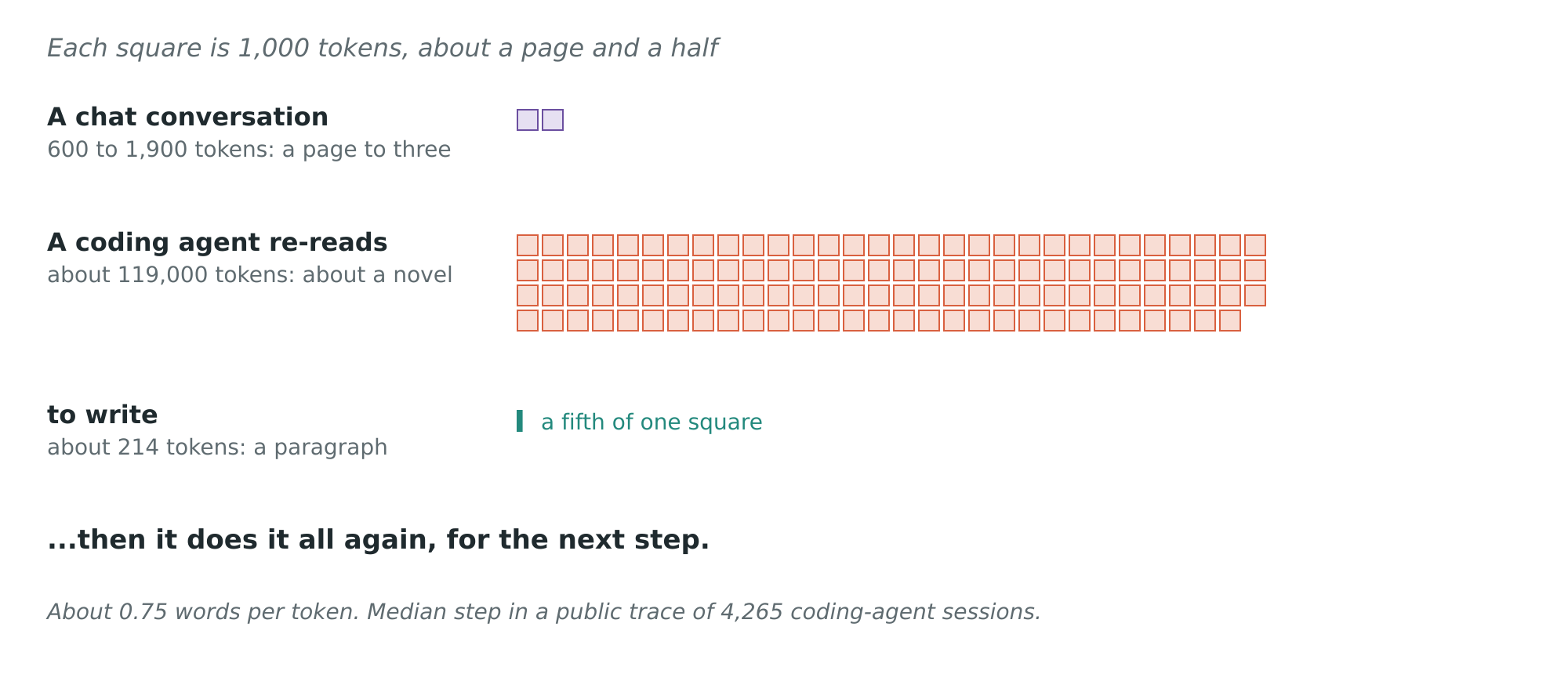
The third is the always-on background agent. It reads every input as it lands: every email, every order, every ticket. Nobody is waiting on any single answer, but it has to keep up, and its context never really resets because the work never stops. Run a business on these and you are running thousands of them at once. What binds here is the working memory, multiplied by how many are live.
The fourth is the overnight batch. No deadline but the morning. It is deferable and easy to pack together, and what it needs is throughput: get through the pile before the staff come in.
Two of these are measured and two are not. The assistant and the supervised agent have public traces behind them. For the always-on agent and the overnight batch I found no public trace of a business agent at all. The nearest are a study of agents run as offline batches (Concur, preprint, January 2026, abstract only) and a day of production logs from coding, search and assistant agents (preprint, August 2026, extract only). I will use the two measured kinds to argue about the two unmeasured ones, and I will say so when I do.
What the four have in common is the direction of travel. The mix is moving from the first kind towards the second and third. Average prompt length per request rose about fourfold in a year, from around 1,500 tokens to over 6,000 (OpenRouter and a16z, December 2025). By the autumn of 2026 agents were taking about 76 to 80 per cent of that platform’s tokens (OpenRouter’s October recap, reported second-hand, and Menlo Ventures, November 2026). It is one developer-heavy platform, counting tokens, not users, and I read most of it as the second kind: a developer watching an agent that runs sub-agents. So it is the early symptom, not the proof, and these are cloud tokens: work done on the shared box, not memory held on yours. It is still the one-line answer to why the data centres keep coming: automation moves the work from the first kind of agent to the second and third, where the context is long, always held, and multiplied by every agent running. I can show that for the coding traces. For the rest it is the direction the public numbers point, not a measurement.
There is a tension here with Thesis 2 that I am not going to smooth over. Thesis 2 said bound the job and keep the model’s context short. Working against it is the everything hammer: one big model is handed every step, so every step re-reads the lot. One peer-reviewed study measured the waste on a coding agent: trimming the context cut the input by 39.9 to 59.7 per cent with no loss in results (AgentDiet, FSE 2026). So the fix is design: fixed code for the fixed steps, then trimming, compaction and short-context sub-agents. The always-on agent is where the opposite bet, that the token streams only get longer, has the most going for it, because its stream is the inflow, and nobody shortens an inbox. I have not settled that reconciliation and I will not pretend to here.
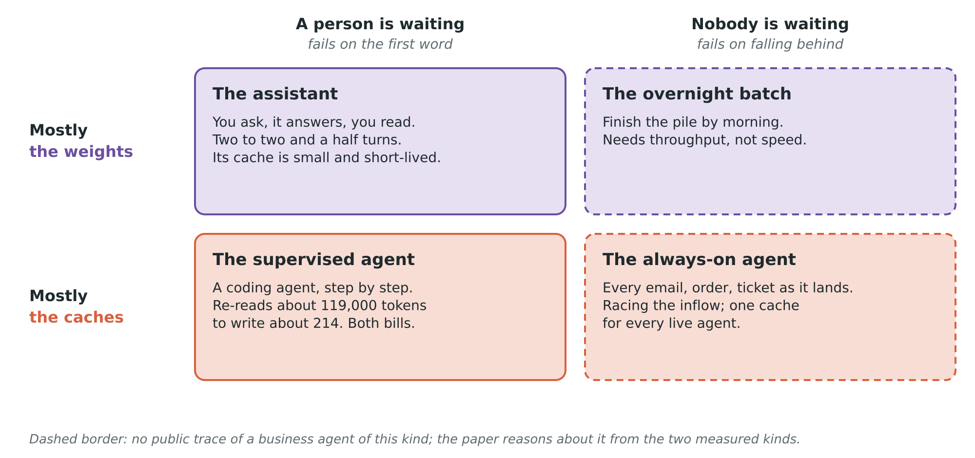
Two of the four have a person waiting. Two do not. That difference hides a second one, and it is the subject of the next section.
“Reactive” means two things
Ask a business what it wants from an agent and the word that comes back is reactive. It should respond when something happens. The word hides two demands, and a box sized for “reactive” without saying which is sized for neither.
The first meaning is a person waiting. You asked, and until the first word appears you are doing nothing. What fails here is the wait before the first word: one answer against one clock. The assistant and the supervised agent live in this meaning.
The second meaning is work arriving. Emails land, orders land, tickets land, and the agent has to keep pace with the inflow. No single answer needs to be fast. What fails here is falling behind. If the box serves work more slowly than work arrives, the backlog grows, and a backlog that grows does not level off. That is a queueing condition, not a speed condition, and the always-on agent lives in it. The overnight batch lives in neither. It only has to be finished by morning.
With agents the queue does worse than grow. On one data-centre node serving a fleet of robot-control agents, throughput fell from about 2.4 requests a second to about 0.6 as the fleet went from 20 to 32, because re-reading old context crowded out the writing (He, preprint, November 2026; measured). The textbook queue only gets slower as it fills. This one goes backwards.
The obvious objection is that I have renamed latency and throughput. Partly. But the always-on agent fits neither term cleanly. An overnight job can wait until tonight. The email agent cannot put its reading off, because it does not know which email is urgent until it has read it. It is racing the inflow.
One more property bites hardest on exactly this kind of agent. Jobs are not the same size. One long email stuck at the front of the queue, and every short urgent one behind it waits, so a box sized on arrivals alone is undersized. There is no public data on the mix of job sizes a business agent sees, so that is reasoning from how queues behave, not a measurement.
Whichever meaning of reactive you are sizing for, the thing you are sizing is memory. The next section says what it is made of. Figure 6 sorts the four agents on both questions.
What agents hold: the model, plus the memory of every conversation
The memory a model needs has two parts, and almost everybody counts one.
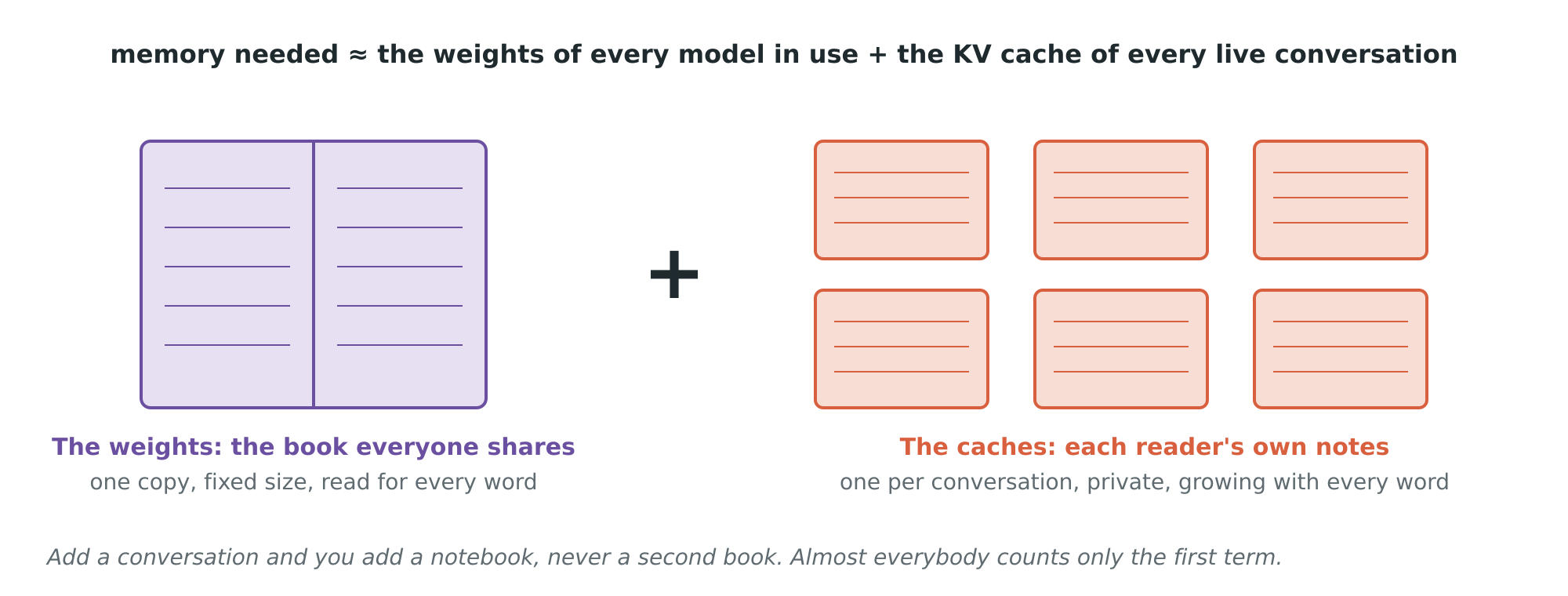
The first part is the weights. That is the model itself, the numbers it learned in training, and it is shared: every user, every agent, every conversation on the box reads the same weights. A 70-billion-parameter model at 16-bit precision is about 140 GB of them. Fixed, known, on the spec sheet.
The second part is the KV cache, and it is the one people forget. As a model reads a conversation it works out, for every token, a pair of vectors it will need again for every token that follows. It keeps them. That store is the model’s working memory of the conversation: its notes on the desk. It is private to each conversation, it grows with every word read and every word written, and it is thrown away when the conversation ends. The weights are the book everyone shares. The cache is each reader’s notes, and each reader has their own.
So the sizing law has two terms (Figure 7):
memory needed ≈ the weights of every model in use + the KV cache of every live conversation
The law is published. Singh derives it for Llama 3 70B at 16-bit: 327,680 bytes of cache for every token, so one conversation outweighs the weights at 427.2k tokens and 32 conversations do it at 13.4k tokens each (Singh, 2026; derived, not measured). And you cannot pack to a hundred per cent: before paged memory, serving systems used only 20 to 38 per cent of their KV memory for the conversation itself (Kwon and others, 2023).
What is mine is the same sum read from a box you own. Tokens drive the cache and model size drives the weights, but the bytes per token are set by the model’s attention design, not by its size.
| Model (attention design) | KV cache per token, 16-bit | One conversation at 32K | One conversation at 128K | Weights | Conversations at 32K before the caches outweigh the weights |
|---|---|---|---|---|---|
| Llama 3.1 8B (GQA) | ~131 KB | 4.3 GB | 17 GB | 16 GB | ~4 |
| Llama 3 70B (GQA) | ~328 KB | 10.7 GB | 43 GB | 140 GB | ~13 |
| DeepSeek-V3 (MLA) | ~70 KB | 2.3 GB | ~9 GB | ~671 GB at 8-bit | ~290 |
Calculated from the published model configurations; DeepSeek’s own ISCA 2025 paper gives the 70 KB figure. Configurations checked 3 November 2026.
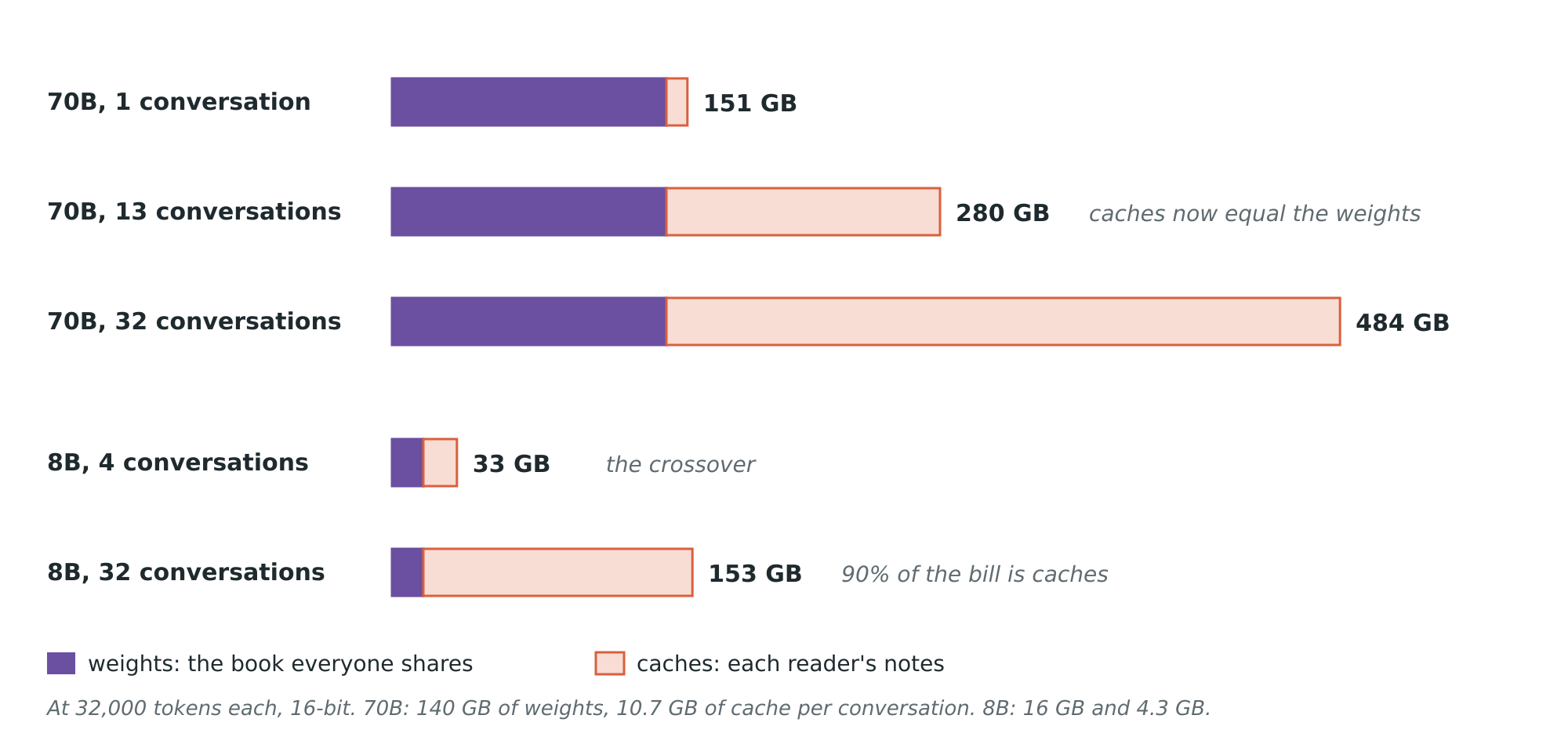
Read the last column (Figure 8 draws it) and the finding that shapes the rest of this paper falls out of it. Shrinking the model cuts the weights far faster than it cuts the cache. The smaller the model, the sooner the conversations become the whole bill: for one 4-billion-parameter model, 7.5 GiB of weights against 9 GiB of cache at four conversations of 16,000 tokens (KVSwap, preprint; computed, not measured). It is the strongest objection to where this paper ends up, and I would rather raise it than have it raised. Act three answers it.
Now put an agent on the box rather than a chat. An agent mostly re-reads. In the coding trace from section 2, 52.56 billion of the 54.90 billion input tokens came from the cache of earlier context, against 186.9 million tokens written. The agent is not writing. It is re-reading its own notes, every step, to write the next line.
The standard answer is that caching makes this cheap. It misses what is being cached. The cache stops the earlier words being worked out again. It does not stop them being held (only a prefix shared between conversations is held once), and it does not stop them being read for every new word: on one data-centre GPU a small model’s energy per token rose from 107 to 242 millijoules as its context grew from 4,000 tokens to 16,000 (Ma and others; the GPU’s own sensor). On a rented API that memory is the provider’s problem. On a box you own it is yours, and it is the expensive part of a small box.
Which brings the two meanings of reactive back. Put several agents on a box that cannot hold every live cache at once, and the box has to choose each time it switches between them. Write the outgoing cache out to the drive and read the incoming one back in, which costs drive writes and time. Or throw the cache away and rebuild it by re-reading the whole context, which costs only time. Wear or wait.
The wait is now measured. On a server with two data-centre GPUs, going from 15 coding agents to 20 took the cache-hit rate from 98.85 per cent to 16.78 and each request’s speed from 30.08 tokens a second to 16.96 (Yuan and others, preprint, September 2026). On an eight-GPU node re-reading stretched a request by up to 7.14 times (ThunderAgent, ICML 2026, peer-reviewed, vendor co-authored). And once on a machine a business might own: an Apple M4 Pro with 10.2 GB for caches held six agents at 4,000 tokens of context and three at 8,000, and evicting one cost a 15.7-second re-read against 0.58 seconds to restore it from the drive (Shkolnikov, single-author preprint, 2026). Wait fifteen seconds, or write to the drive. How large the wait grows on a business box under real work is still my reasoning. So is the wear (section 8.4).
One point in the other direction, because it is a tailwind and not a threat. The labs are cutting the cache hard, and every cut moves the crossover, not the slope (section 8.7).
That is what the memory holds. Why memory and not maths is the question underneath, and it is a question about physics.
Why memory, not maths: the fetch
A model writes one word at a time. To write each one it reads its active weights, and the conversation so far, out of memory, and does a very small amount of arithmetic on each number it read. Then it does it again for the next word. The chip is not thinking. It is waiting.
Put a meter on it. Speed is the memory’s bandwidth divided by the bytes read per word. Energy is those bytes times the cost of moving each one, plus whatever the box burns standing still while it waits. Bytes read per word, the active weights plus the conversation’s cache, is the measure this paper runs on. Figure 9 draws the fetch.
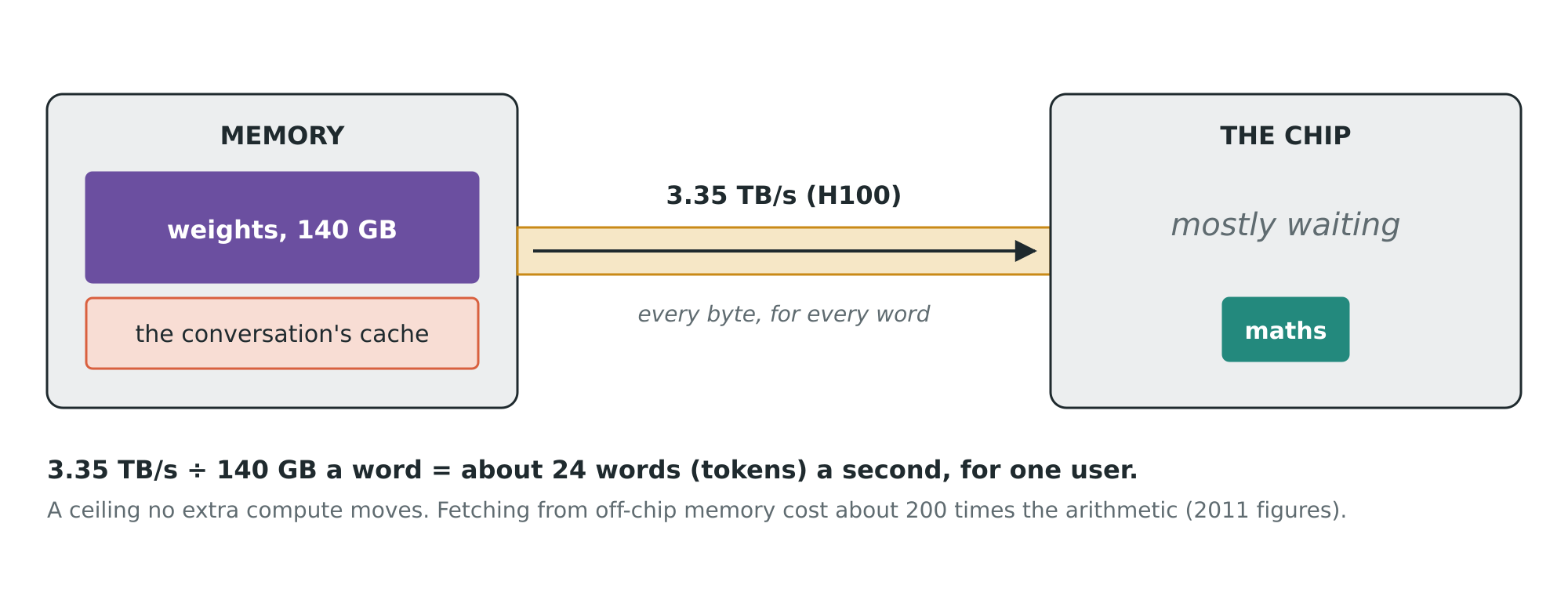
That decode is bound by memory and not by maths is published (Singh, 2026), and the sum fits on one line. A 70B model at 16-bit is about 140 GB of weights. An H100 reads its memory at 3.35 TB/s. Divide one by the other and you get about 24 tokens a second (NVIDIA’s published figures; the sum is mine), a ceiling for one user that no amount of extra compute moves. The fastest chip does not even reach it: serving one user, an H100 ran at 0.270 of what its bandwidth allows and a slower L4 at 0.810 (Chen, preprint, May 2026; measured on a 7B model). Slower memory is used better. Beyond 7B that is my reasoning.
Moving is the dear part. On figures from 2011, fetching the operands from memory off the chip cost about two hundred times the arithmetic done on them (Keckler and others; NVIDIA authors). The two trips that matter here cost nearly the same: memory stacked beside a data-centre chip and the memory in a business box cost about the same to read, 3.4 to 4.5 picojoules a bit on the makers’ own figures, which do not all draw the boundary in the same place. An SSD costs thirty to nearly fifty times that. The energy goes into charging the wire, and high speeds force short wires, which is why the fastest memory sits beside the chip. So the box does not draw less because its bits are cheaper. It draws less because it moves fewer of them.
One run shows it on a desk. In a test published in July 2026, a Mac Studio writing with a dense 27-billion-parameter model drew 138 W and wrote 21.5 tokens a second. With a sparse model that reads about 5 billion parameters per word it drew 94 W and wrote 74 (one author’s measurement with the author’s own tool, checked against a wall meter; not peer-reviewed). Fewer bytes per word: faster and cooler at once. The electricity is a fraction of a penny an answer, so the watts matter as the cap, not the cost.
Now the concession, and I will never state the claim without it. Hyperscaling works. A data-centre GPU serving hundreds at once fetches the weights once for all of them; for a dense model on an H100 the weights stop being the limit near 295 sequences in flight (Singh, derived). On one B200 a 32-billion-parameter model has been measured at 0.15 to 0.31 joules a token (Chung and others, preprint; the GPU alone), against 6.4 for the dense model on the desk: different models and different meters, so I hold the size of that gap loosely and its direction firmly. A batched data centre beats the box per answer. Britain cannot get that answer (section 10), and the hyperscalers are meeting limits of their own (sections 6 and 7).
Two things batching does not rescue. The first is attention. The cache is private to each conversation, so its share of the work stays memory-bound however large the batch (Recasens and others, IEEE CLOUD 2025, peer-reviewed; measured on an H100 with a 1.3-billion-parameter model). The notes on the desk do not get cheaper by having more desks. The second is the sparse model, which does less maths per token and holds no less memory (section 8.1). Yuan and Long derive a “MoE tax” of 32 times, which puts DeepSeek-R1’s crossover near 4,700 users on one H100, more than an eight-GPU node can hold (derived, by authors who sell a rival chip). The router chooses per token and per layer, so a mixed batch wants nearly every expert. That step is my reasoning, and section 12 uses it: group the work by task and some locality returns.
If every token is a trip to memory, the obvious move is to shorten the trip. The industry has been shortening it for decades, and the next section is where that road ends.
How memory was moved closer, and where that ends
From 1946 to 2009 the work a computer did per unit of electricity doubled every 1.57 years (Koomey and others, 2011). The rule behind it was Dennard’s of 1974: shrink every dimension and the voltage together, and each part does the same job on less. Then the voltage stopped falling, because transistors that small leak (Horowitz, 2014), and by Koomey’s later count the doubling slowed to every 2.6 years. A hundredfold a decade became sixteenfold.
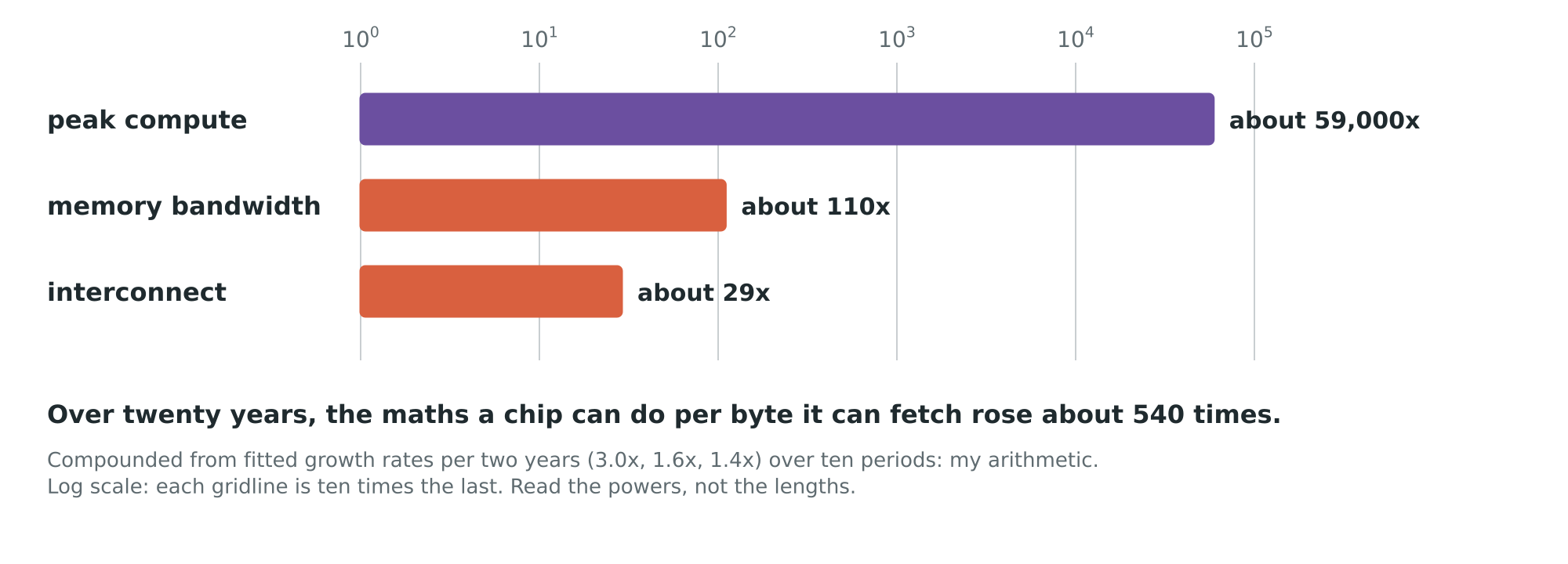
The shrinking was never even. Logic gained more than wires did, so the sums got cheap and the trip did not. Wulf and McKee named the result the memory wall in 1995, and it never closed: over the twenty years to 2024, peak server compute grew 3.0 times every two years while memory bandwidth grew 1.6 times and interconnect 1.4 (Gholami and others, 2024, peer-reviewed; fitted trends). So the industry moved the memory closer. Figure 10 shows how far the gap has opened.
First it stacked the memory beside the chip, on the same package, which is how an H100 reads 80 GB at 3.35 TB/s. Then it put the memory on the chip. Cerebras uses a whole wafer as one chip, with 44 GB of SRAM on the same slab as the cores, read about 6,400 times faster than the H100 reads its memory (Cerebras’ figures; the ratio is arithmetic). That is the end of the road, and it is sold to the hyperscalers as speed. It is no escape for anyone else: in October 2026 no model in Cerebras’ public catalogue fitted one wafer at 16-bit.
Each step closer costs more than the last, and the buyers who can pay are meeting limits too. Stacked memory rose in price by about a third between 2023 and 2025 while ordinary memory nearly halved (Ma and Patterson, 2026, Google authors). In November 2026 NVIDIA’s own pages gave its next GPU, Rubin, 19.2 TB a second, where its earlier announcements had promised up to 22.
The box a business can buy made the opposite trade: capacity at the price of bandwidth. A Mac Studio reads up to 512 GB at 819 GB/s on the M3 Ultra of March 2025 and at 1.2 TB/s on the M5 Ultra of August 2026: a quarter to a third of an H100’s speed, from six times the capacity. Bandwidth has grown, only more slowly. The shortage shows in the price. Apple withdrew the 512 GB option in March 2026 and brought it back on 28 October 2026 on a different machine, the M5 Ultra, where the memory option alone cost $15,500 against $4,000 before (press reports of Apple’s prices).
That machine met the test I once set for changing my mind: about 500 GB at about 800 GB/s at a price a business could pay. It strengthened the small box, because one business can now hold a far bigger model. What it cannot do is serve thousands of live conversations at speed, because the limit was never the weights. It was the caches. So the test is now a ratio: capacity at bandwidth that keeps pace with demand, at a price one business can pay. Bandwidth has grown 1.6 times every two years; prompt length per request, the only demand figure I have, rose about fourfold in one year (section 2). I have no dated series for tokens per agent, so the ratio is unpriced, and I say so.
Plant one thought here and leave it for act three. A 27B model at 8-bit, about 31 GB, fits in 44 GB with room to spare. Shrink the model until the whole of it fits the memory you have, and the wall never fires. That is not where the industry went. It is where this paper goes.
That is the memory. Act one has one section left, and it is where the physics first touches a person.
Why it fails in production: the wait before the first word
The memory wall does not show itself to a user as a number on a spec sheet. It shows itself as a wait. You ask, the cursor blinks, and nothing comes. That wait is where agents fail in production, and they fail at a point the lab never sees.
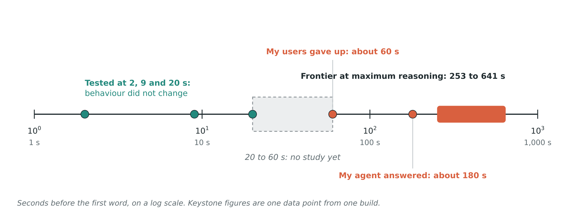
The wait before the first word has two factors: how many tokens the model thinks before it starts answering, and how long each of those tokens takes. Multiply them and you have the wait. Streaming speed, the thing people measure, is almost never the problem. Adults read at about five or six tokens a second (Brysbaert, 2019), and in November 2026 the models Artificial Analysis tracked streamed at 14 to over 1,600. Nobody is waiting for the words to appear. They are waiting for the first one. At maximum reasoning effort, the frontier models that hide their reasoning took between about four and eleven minutes to produce it (Artificial Analysis, November 2026, 253 to 641 seconds). The thinking is what you wait for.
Because the wait has two factors, the fix works on both. Code does the heavy lifting, so the model has less to think through: fewer tokens. And a smaller model, preloaded and resident, makes each token faster: less time per token. Do one and you cut the wait. Do both and you change what the product is.
I learned this the expensive way. An earlier version of the scheduling agent I built at Keystone failed user testing on exactly this wait. It often took about three minutes to answer. A user mid-workday, watching the cursor, gave up after about one and did the reschedule by hand, and nearly all of the wait was the model thinking rather than the system fetching data. You cannot test a model people will not wait for, so the wait did not just hurt the product. It stopped the testing. That is one data point from one build, and I present it as one data point.
The one controlled study I can find points the other way, and it deserves stating in full rather than waving off. A CHI 2026 experiment with 240 participants held streaming speed fixed and varied the wait before the first token across 2, 9 and 20 seconds. Behaviour did not change, and the two-second answers were rated less thoughtful than the slower ones. Only at 20 seconds did some begin to lose patience. The study stopped there, and I have found none that tests further. My users left at 60. Nobody has published where between the two the failure point sits. I read that as a gap in the evidence, not a result against the claim. Figure 11 puts every wait in this section on one scale.
Thinking less is not always thinking worse: on hard maths questions the shortest of twenty answers beat the longest by up to 34.5 percentage points on one model’s average (Hassid and others, preprint, measured). Where to bound the thinking is a routing decision (section 12).
Here is how the wait and the memory connect, in three steps, and the three steps are the spine of this paper.
First: production exposes the wait that development hides. A developer sits through a minute; a user does not. A data centre can buy its way past the wait with scale. A box you own cannot. Second: more agents means more caches. Batching shares the weights and never the caches, so as agents are added either the tokens slow, because the bandwidth is split more ways, or a cache has to leave the box for the drive. Third: on a fixed box, shrink what each agent holds. A smaller model leaves room for more caches, and code doing the heavy lifting keeps the contexts short, so each cache is smaller too. That is act three, and act two is the ground it has to be earned on.
One thing I want to say as a bet rather than a finding, because said as a finding it explains away the 20-second study too conveniently. I think the wall has not been seen at full strength yet. The second kind of agent already burns most of the tokens on one developer-heavy platform (section 2). That is the early symptom. The third kind, always-on agents at production scale, will meet the same wall harder, because nobody bounds their sessions, and a longer session is a bigger cache (Singh derives that; the coding traces measure the contexts). That last step is a bet, and I lose it if the always-on agents arrive and the wall does not.
One sign the bet is not empty, given with its weakness attached. Memory was short before the agents arrived, and it is one shortage: the stacked memory beside a data-centre chip and the RAM in a laptop are both DRAM. Conventional DRAM contract prices rose by roughly 93 to 98 per cent in the first quarter of 2026 alone (TrendForce, June 2026). On its earnings call of 28 October 2026 an SK hynix executive said, through an interpreter, that its DRAM and stacked memory were “effectively sold out” through 2029; the company’s own release says only that contracts cover more than half of its 2027 and 2028 capacity. The hyperscalers’ answer works, and they are queuing for it too. That shortage comes from the data-centre build-out, not from agents. But memory is dear because the hyperscalers are buying it, and the same scarcity raises the price of the box in your server room.
So act one ends with the four questions set. A method for cutting the memory has to keep the model on the box: memory. Keep the first word coming inside the time a person will wait or the inflow allows: wait. Not destroy the hardware doing it: wear. And give back an answer that survives: quality. Act two puts eight methods through them.
Act two: eight ways to cut the memory, judged from your own box
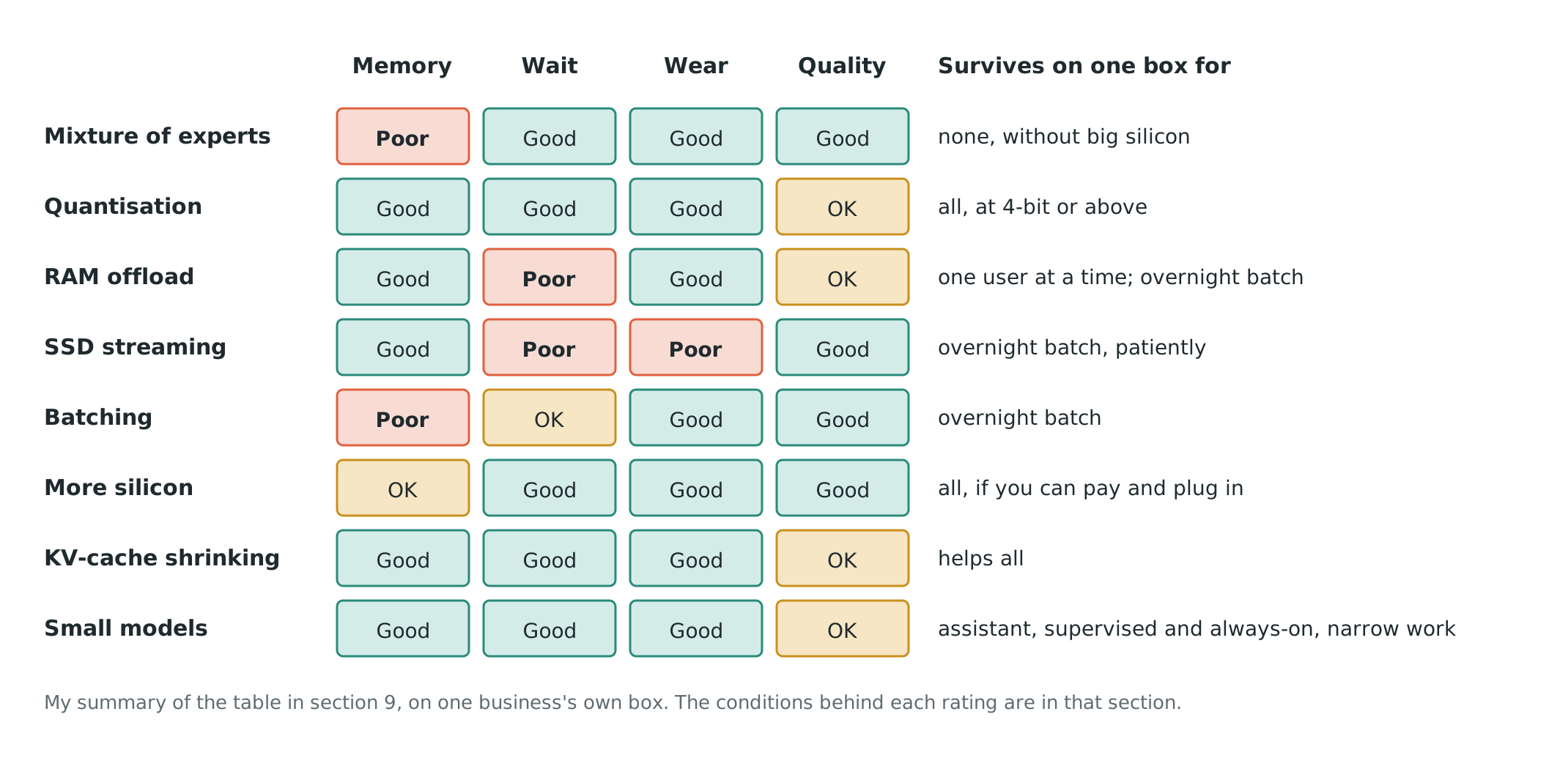
Every method in this act is real, deployed somewhere at scale, and works. That needs saying first, because the easy version of this paper would sneer at them, and the easy version would be wrong. Together they are the industry’s version of the third lever: squeeze the data at every step. What follows is where each one breaks, on one box, when the workload stops being one developer and becomes a business. Each gets the same beats: what it is, why it works in development, where it breaks on your box. Section 9 scores all eight on the four questions. Figure 12 gives the overview first: all eight, scored on the four questions.
Eight methods
8.1 Mixture of experts: fire fewer weights per token
What it is. Split the model’s feed-forward layers into many parallel blocks called experts, and put a small router in front of them that picks a few per token, per layer. Only the picked experts do arithmetic. DeepSeek-V3 is the usual example: 671 billion parameters in total, 37 billion active for any one token.
Why it works in development. Less maths per token, so each token is cheaper and faster to produce. One of the cheapest capable models to call in November 2026, DeepSeek V4.1 Flash, at $1.20 per million output tokens at peak, stored 763 billion parameters and used 16 billion of them for each token it wrote.
Where it breaks on your box. Every expert has to be housed. The router can choose any of them for the next token, so all of them must sit in fast memory whether or not they fire. The model thinks like a 37B model and is housed like a 671B one. DeepSeek’s own decode deployment ran across 144 GPUs in 18 nodes (its infrastructure note, March 2025), and Yuan and Long derive that an eight-GPU node serving such a model uses about 0.6 per cent of the arithmetic it paid for (derived, by authors who sell a rival chip). The mixture of experts saves on a bill you were not really paying, the compute, and leaves untouched the one you were. Figure 13 shows it.
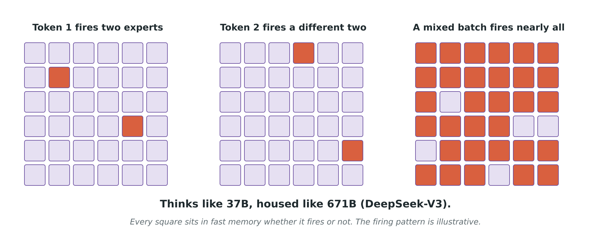
The counter you will hear is that DeepSeek’s memory bill did fall. It did, and it is worth being exact about which bill. Its cache per token is 86.4 per cent smaller than Llama 3.1 405B’s (70 KB against 516 KB in DeepSeek’s ISCA 2025 paper; the percentage is my arithmetic). That is the second term of the sizing law. The first term, every expert resident, did not move, and that is the bill that decides who can own the thing. DeepSeek is among the cheapest models in the world to call and among the most expensive open models to own.
8.2 Quantisation: fewer bits per weight
What it is. Store each weight in fewer bits. Sixteen is the training precision; eight halves the memory; four halves it again. Fewer bits per weight also means more weights through the same memory bandwidth, so quantisation buys memory and speed together.
Why it works in development. The weights shrink, and a smaller read is a faster token. The headline demonstration is Unsloth taking DeepSeek-R1 from 720 GB to 131 GB, a fivefold cut (Unsloth, January 2025).
Where it breaks. On quality, not memory, and the break is a staircase with a cliff at the bottom. Eight-bit is close to free: lossless across the whole Llama 3.1 family in the largest study, over 500,000 evaluations (Kurtic and others, ACL 2025; its authors sell quantised models). Four-bit weights cost about half a point to four points, depending on the task and the model (the same study, and ACBench, ICML 2025; both measured and peer-reviewed), and far more at long context: up to 59 per cent in the worst case measured (Mekala and others, EMNLP 2025). Three-bit costs more than seven per cent of reasoning accuracy at 8B and 70B (Liu and others, COLM 2025). Two-bit, squeezed after training, collapses. Figure 14 draws the staircase.
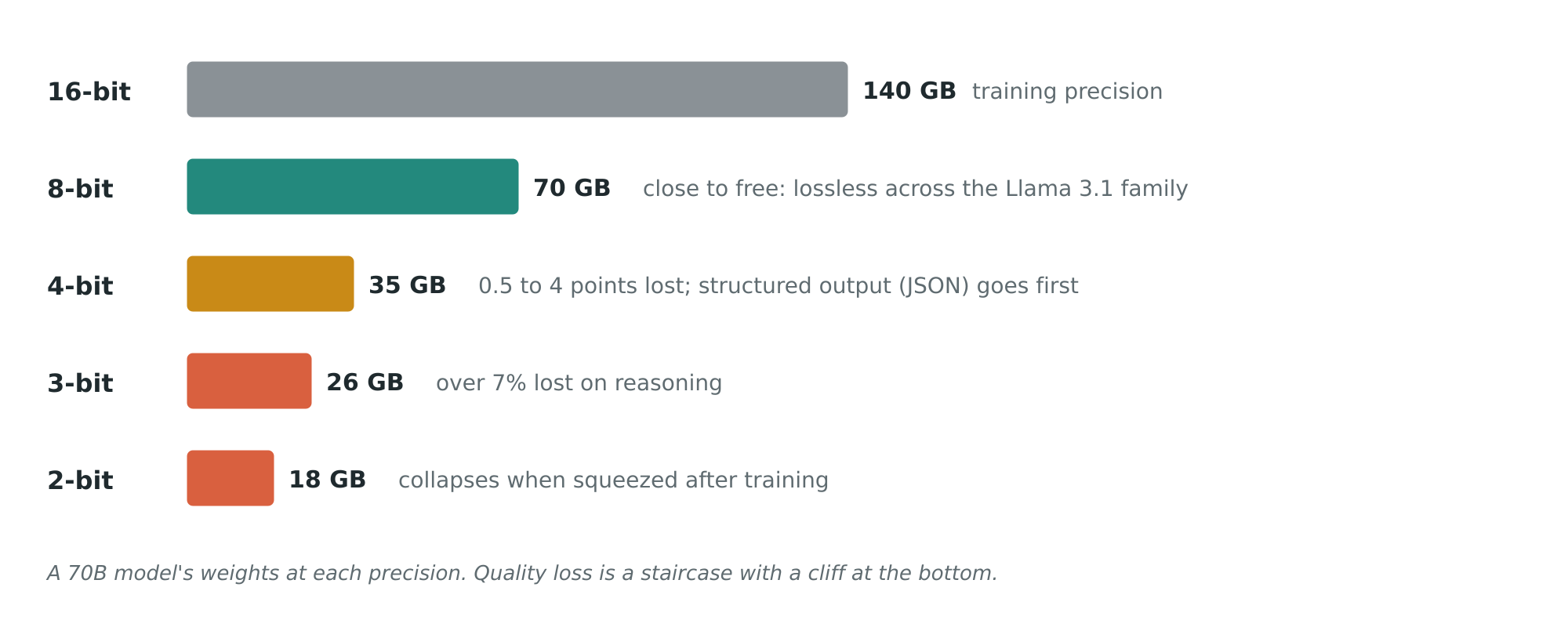
The losses are not spread evenly. Plain tool calling broadly holds at 4-bit: ACBench measured 0.4 to 3.6 points lost on a 7B model. What goes first is structured output, the JSON a model hands to the code around it, and some multi-step tasks. That is the joint between the model and the deterministic tools, and on a box you own it has to be guarded, with constrained decoding and validation, not assumed.
The Unsloth counter is the one to hold: DeepSeek-R1 runs at 1.58 bits. It runs. Running and keeping quality are not the same thing. On the one quality test Unsloth published it scored 69.2 per cent against 91.7 for the 2.22-bit version, with its attention kept at four or six bits. It shows where the bits should go, not a frontier model at 1.58 bits.
The credit for putting a 671B model on a desktop belongs here, to bit-width, not to the mixture of experts. Sparsity buys compute. Quantisation buys memory.
8.3 Offloading to system RAM
What it is. Keep the attention layers and the busiest experts on the GPU and park the rest in ordinary system memory, pulling an expert across when the router asks for it. KTransformers runs the full 671B DeepSeek-R1 at 4-bit on 14 GB of GPU memory plus 382 GB of RAM, at roughly 9 to 14 tokens a second (the project’s own figures, 2025).
Why it works in development. One user generating one stream reuses the same handful of experts across adjacent tokens, so a small cache of experts on the GPU hits often enough that the slow trip to RAM is rare. For one person at a keyboard, it is a frontier model on a workstation.
Where it breaks on your box. At the second agent, for anything a person is waiting on. Put a batch of different users’ tokens through together and they collectively route to nearly every expert, the cache stops hitting, and you are back to needing all of them in fast memory. The mechanism is published: decode latency scales with the experts activated across the batch, not per input (Lynx, preprint, 2024; read in abstract only). ExpertFlow measured the fall on a small model: a plain cache of 16 experts went from a 76.6 per cent hit rate at a batch of 4 to 58.4 at a batch of 16 (DAC 2026, peer-reviewed).
It survives where nobody is waiting. MoE-Lightning ran Mixtral 8x7B on one 16 GB GPU with the experts in system memory and reached up to 10.3 times the throughput of earlier systems (ASPLOS 2025, peer-reviewed, measured): about 30 tokens a second across 504 sequences, some 0.06 each. That is an overnight batch, not a conversation. It is consistent with this paper, not proof of it.
8.4 Streaming from the SSD
What it is. Go one tier further down. Put the weights, and sometimes the KV cache, on the solid-state drive and stream them in as needed. It is a cliff rather than a slope: GPU memory reads at 2 to 3.35 TB/s, a fast NVMe drive at about 14 GB/s, and that is its sequential rating.
Why it looks like it works. The drive is enormous and cheap, and a demonstration exists: an engine called Colibri streams a 744-billion-parameter mixture of experts from NVMe on hardware that could never hold it.
Where it breaks splits in two, and the two halves fail different questions.
Weights from the drive fail on wait and on energy, not wear. Reading barely wears a drive. What it does is take time: Colibri’s own README gives 0.05 to 0.1 tokens a second on a laptop. A 35 GB model read whole for every word gives one word every two to five seconds, and the drive alone spends 19 to 27 joules on it (arithmetic on Samsung’s datasheet ratings): more than the whole box in section 5 spent per word with its model in memory. A simulation puts streamed expert weights at roughly 4 to 12 times the energy per token of stacked memory (Kyung and others, IEEE Computer Architecture Letters, 2025; simulated, part-funded by Samsung). Streaming whole weights from an SSD is proof that a model can be made to run, not a way to run one.
The KV cache on the drive fails on wear. It lands there when RAM runs out and the system swaps, or when a session’s cache is saved between turns. Whether that wears the drive out depends on the pattern, and anyone can check the mechanism against a drive’s own specification. A shared prefix, written once and read many times, is survivable. A per-session cache rewritten as the context changes is not, on a small drive: one agent on Llama 3 70B rewriting a 128,000-token context two hundred times a day writes about 8.6 TB, roughly thirteen times the daily budget of a 2 TB consumer drive, and would use up its five-year warranty in about 140 days (calculated from the per-token cache size and Samsung’s published endurance for the 990 Pro; the write pattern is assumed). Figure 15 sets the writes against the drive.
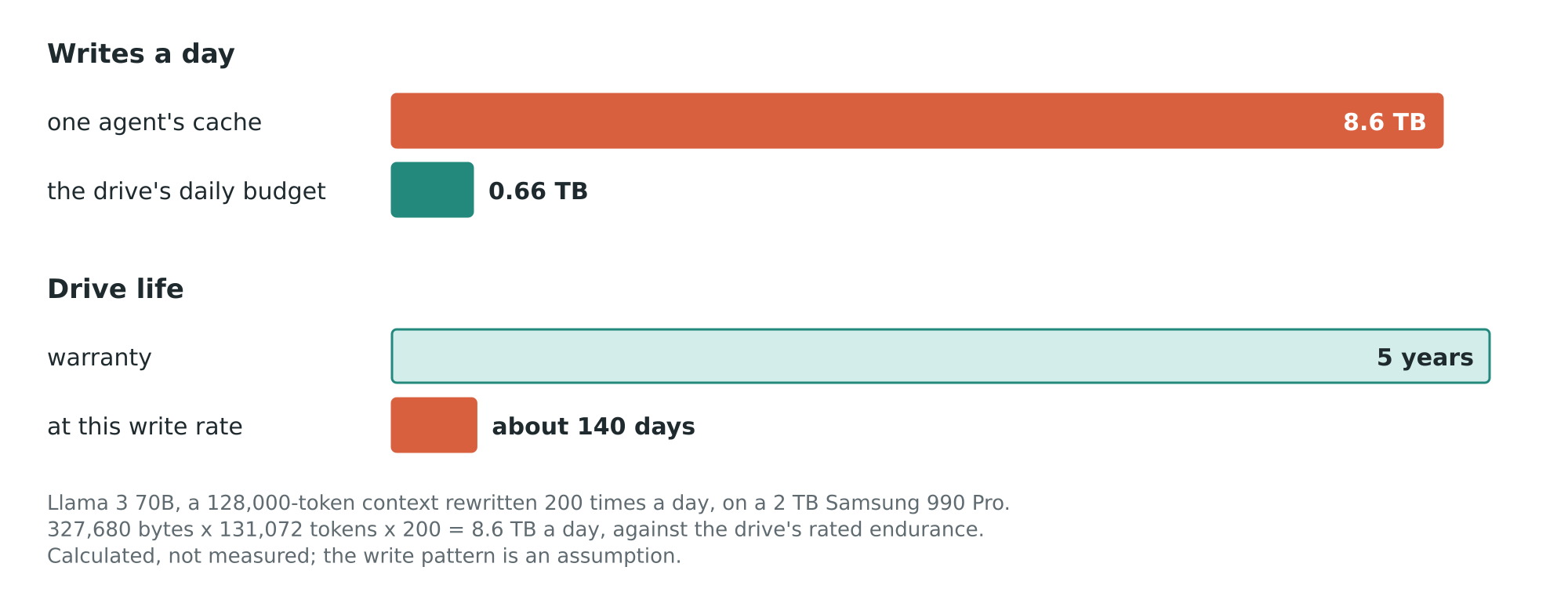
Nobody has measured that wear on a consumer drive. Every figure I can find is computed from rated endurance and none is read from a drive, including the nearest estimate at data-centre scale: 0.2 to 0.4 years of drive life (Gandalf, preprint, October 2026, a storage maker among its authors). Google’s authors rule flash out, on endurance, for a cache updated at every token (Ma and Patterson, 2026). So for the multi-agent box this is the wear half of section 4’s choice, and I label it as before: reasoning from mechanism, not measurement.
8.5 Batching
What it is. Put many users’ tokens through the model together, so one read of the weights serves all of them. For a dense model on an H100 the weights stop being the limit near 295 sequences in flight (section 5).
Why it works. For once, it works in production and not only in development. This is how the providers serve the world, and it is the overnight batch’s home ground. Concede it flatly: for anyone serving many users on big silicon, batching is the answer, and it is a good one.
Where it breaks on your box. Three times. Batching shares the weights and never the caches, so the more users you batch the more caches you hold. A sparse model stays memory-bound at any batch one box can hold (section 5). And you cannot batch your way past the ridge on a box that holds one copy of the weights and little else. Batching is a method for people who already have the memory. It does not get you the memory.
8.6 More silicon
What it is. Spread the model across hundreds of GPUs and shuttle the tokens between them, each GPU holding roughly one expert. DeepSeek’s report specified 320 GPUs across 40 nodes; production ran 144 across 18. Cerebras is the extreme case of the same answer, not its opposite: 44 GB a wafer does not hold a frontier model, so the model is sliced across wafers and the traffic the wafer exists to abolish comes back between them.
Why it works. It is rational for anyone who batches, and I will not pretend otherwise. If you will not compromise on throughput, and the hyperscalers will not, the only way to hold 671 billion parameters in fast memory is to buy enough fast memory. That answers the question the paper opened with: everyone needs so many data centres because the industry’s answer to the memory bill is to pay it, in silicon.
Others have proposed different answers, in simulation, on paper or as a maker’s estimate. I have found none deployed at scale and shown to work. Processing inside the memory is one: a simulated design reports 2.3 times less energy and 5.2 times the tokens per dollar of GPUs (CENT, ASPLOS 2025), and Samsung’s version has been found only in test systems. Yuan and Long meet the same on-premises diagnosis as this paper with different silicon: a decode card holding 512 GB at 819 GB/s for about $19,000 built (their own estimate, for the chip they sell). Their answer is to buy different silicon. Mine is to shrink the model.
Where it breaks. Only on who can afford it, and on where it can be plugged in, which is section 10. It is not an on-prem method, and that is the point of listing it.
8.7 Shrinking the KV cache
What it is. Change what the model stores per token. Grouped-query attention shares key-value heads across several query heads; DeepSeek’s MLA compresses the pair into one small latent vector; the cache can be stored at 8-bit or lower. DeepSeek’s V4-Pro needs, by its own report of April 2026, a tenth of the cache V3.2 did at a million tokens.
Why it works in deployment. The major open families use grouped-query or latent attention. Of all the methods in this act, it is the one that attacks the second term directly.
Where it breaks. Smaller per agent is still one per agent, and still growing with every always-on stream. How much it buys depends on which side of section 4’s crossover you sit: for a 2-bit cache on Llama 3 70B at 128,000 tokens on a B200, Singh derives a bound of 1.25 times the speed for one conversation and 4.82 times for a batch of 32 (derived, not measured). Nor is a squeezed cache free at long context: on one model, NVIDIA’s own evaluation found five to ten points lost on a 128K retrieval benchmark with an 8-bit cache (technical report, February 2026).
For this paper it is a tailwind, and I am not arguing against it. Every lab cut to the cache lets a fixed box hold more conversations. I would rather the labs kept going.
8.8 Small language models: need less to begin with
The first seven methods squeeze a big model or buy memory for it. This one needs less memory to begin with, and it pays in capability rather than in wait, wear or quality.
What it is. A model of a few billion to a few tens of billions of parameters, fine-tuned to a domain or a task, resident on the box in full.
Why it works. On narrow work, it wins. Of 310 small models fine-tuned to their task, 224 beat GPT-4 on it (LoRA Land, 2024, against GPT-4 given at most one worked example); a 7B text-to-SQL model beat a GPT-4 pipeline on the Spider benchmark by 1.3 points (2025). NVIDIA researchers estimate that 40 to 70 per cent of the calls in three agent systems could go to a small model (Belcak and others; a position paper, no experiment). Each win comes with a condition I will attach every time: the task has to be narrow enough for code to do the heavy lifting. The model makes the one judgement the code cannot; the code does the rest. That was Thesis 2’s architecture, and it is the only shape in which a small model’s capability is enough.
Where it breaks. On broad reasoning. GPT-4 beat BloombergGPT on most finance tasks; GPT-4 with careful prompting alone beat the medical specialist Med-PaLM 2 (2023). Specialists win where the task is defined and lose where it is open. And per gigabyte the best general model is still big, sparse and 4-bit, not small and dense. In November 2026, on version 5 of the Artificial Analysis index, the best released model that fitted 44 GB scored 20, the best that fitted 128 GB scored 28 (squeezed to 2-bit), and the best that fitted 512 GB scored 32. Twelve times the memory bought about twelve points.
One more break, and it is the one section 4 promised to return to. With several agents on the box, a small model’s bill becomes mostly cache. The weights shrank; the notes on the desks did not. A small model makes the second term the whole bill sooner. That is why act three cannot say “use small models” and stop. It has to say what each agent holds.
Where every method breaks: the same place
Lay the eight side by side and the pattern is hard to miss. Every one works in development and breaks at a named point on a real box, and most of the named points are the same point: more than one agent at once. Figure 12, at the start of this act, summarises the table.
| Method | Memory | Wait | Wear | Quality | Survives on one box for which agents |
|---|---|---|---|---|---|
| Mixture of experts | unchanged | better | none | unchanged | none, without big silicon |
| Quantisation | much better | better | none | free at 8-bit; small at 4, structured output first; costly below | all, at 4-bit or above, if the task survives |
| RAM offload | much better | one user only | none | as quantised | the assistant, one at a time; the overnight batch |
| SSD streaming | best | worst | weights: none, but dear in energy; per-agent caches: high | unchanged | overnight batch, patiently |
| Batching | cache grows per user | good on big silicon | none | unchanged | overnight batch |
| More silicon | buys it | good | none | unchanged | all, if you can pay and plug in |
| KV shrinking | better per agent | better | less to swap | small, worst at long context | helps all |
| Small models | least | fastest | none | full on narrow work, short on broad | assistant, supervised and always-on, when the work is narrow |
Notice what all eight have in common. Each cuts what one step costs. None asks how little the job needs, and the total keeps rising.
One correction, stated so it is not lost. These methods are deployed at scale. What is not deployed is the lean version on one box, because the lean version breaks at concurrency, and the fix for concurrency is hundreds of GPUs. That is where the industry really stands, and it is exactly the position a business in Europe cannot take, for the reason act three begins with.
Act three: the alternative
Act two ended with the industry’s answer: pay the memory bill in silicon, and if one box cannot hold the caches, buy a building that can. Act three is what you do when you cannot.
The shared data centre is a bigger box that everyone shares
Cloud does not sell compute. It sells the right to scale: the right, but not the obligation, to take more capacity when you need it, with the premium for that right folded into every hour you buy. For a spiky, unpredictable workload it is worth every penny. For a steady set of always-on agents it is a premium on an option you never exercise, and when everyone runs always-on agents there is nothing spare to scale into. A shared data centre is a bigger box that everyone shares. Its memory wall is the same wall, met at a larger scale, by everybody at once.
That is the first lever, scale, and it needs a grid connection. In its evidence to Parliament in May 2026, Britain’s system operator had about 5 GW of data centres connected by 2030 on its ten-year forecast (NESO). Behind that sat a queue of about 73 GW (Ofgem, July 2026). Perhaps half of that queue is speculative; the operator’s own slides of September 2026 are reported to put it at close to half. It does not matter which half. A firm that needs the capacity this year is not getting it from a queue. Figure 16 draws the queue against one socket.
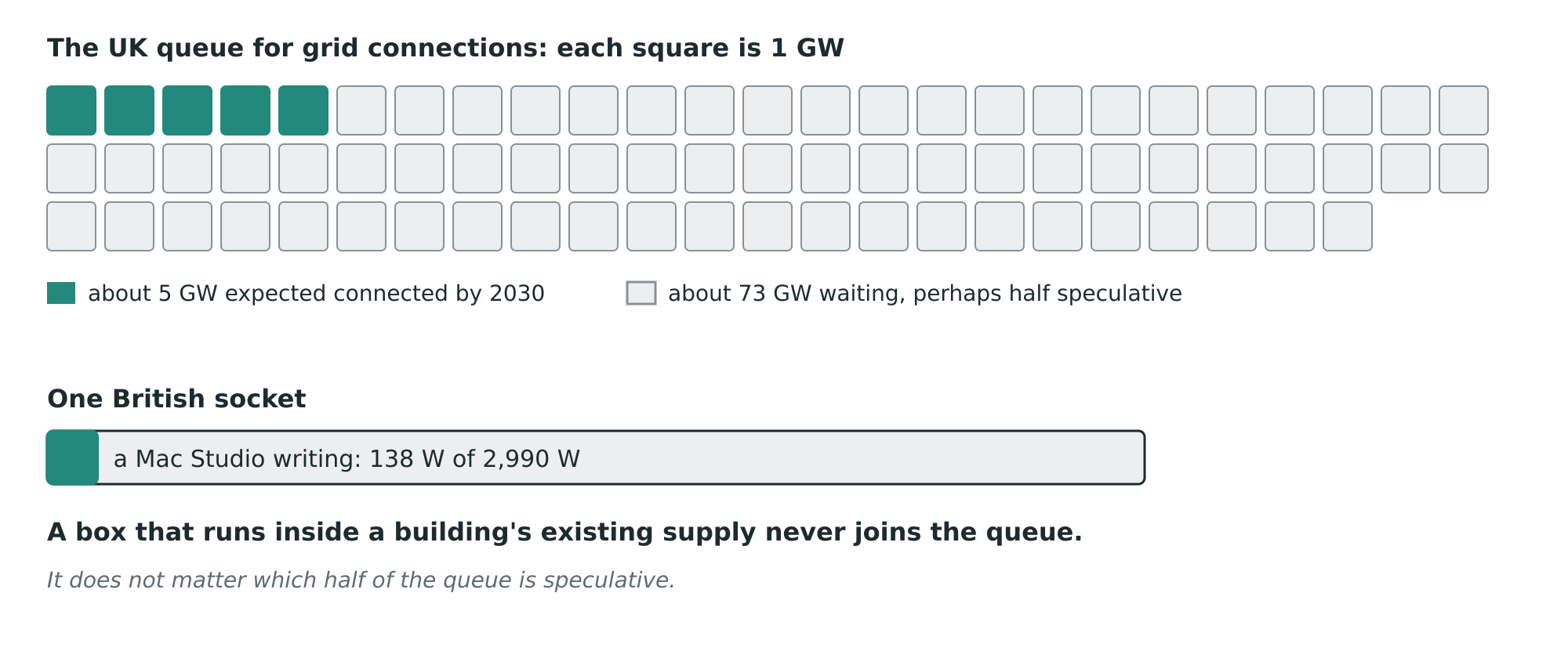
And some of what could connect is pausing on price. Only about 40 per cent of the British data-centre capacity Ofgem had identified had reached a final investment decision (February 2026), and OpenAI paused its UK build in April 2026, saying it would move forward “when the right conditions such as regulation and the cost of energy” allowed. Nor is the wall only British: Texas paused its studies of large new loads in August 2026 with about 474 GW waiting (ERCOT). A sovereign data centre, the thing European governments announce, joins that queue at the back.
Which produces the one move this paper is about. A model small enough to run inside a building’s existing supply never joins the queue at all. Not further up the queue. Not in it. The desk machine in section 5 drew 138 W while it wrote, from a socket rated for 2,990. Sovereignty over the model starts when the model fits the box you can buy. Sovereignty over the power starts when the load fits the supply you already have. The deployment has to be small enough to sit inside both.
One principle: hold the memory, reshape the work
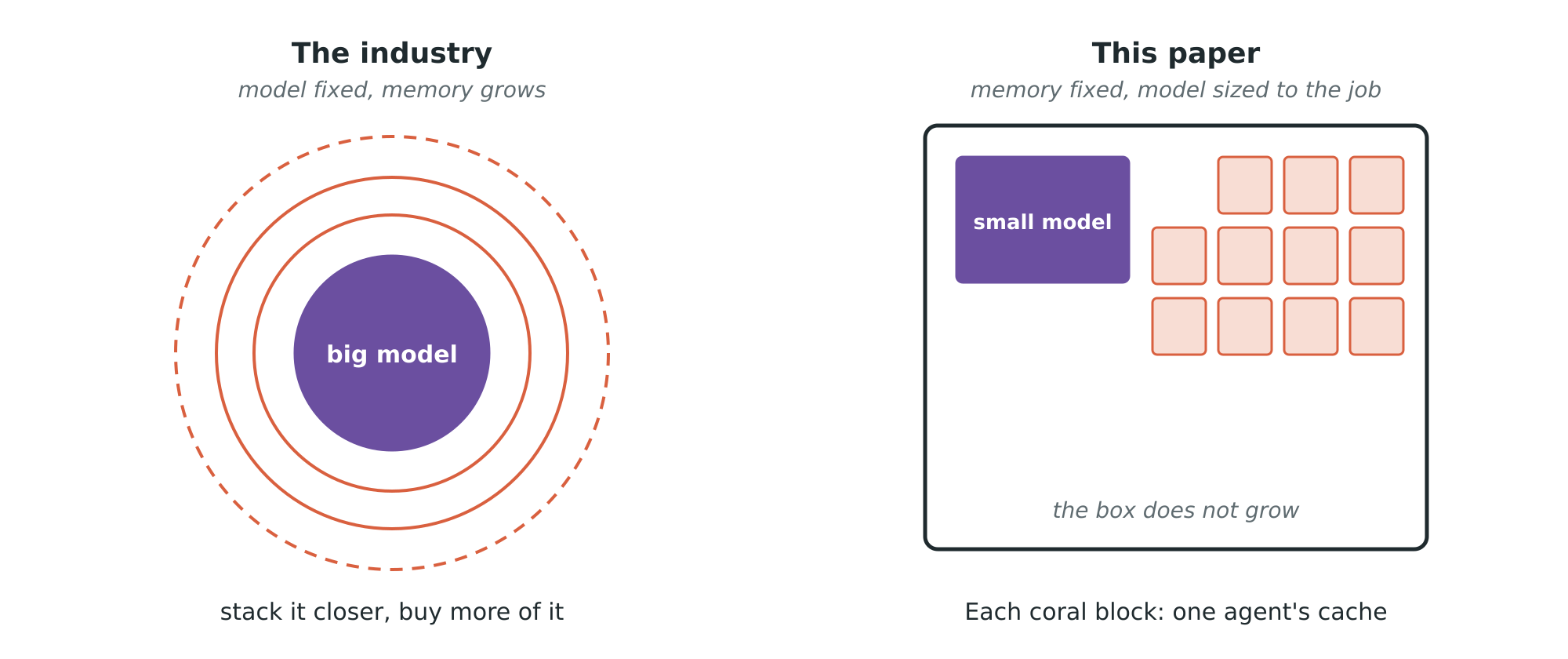
Everyone else in this paper changes the memory to fit the model. Stack it closer, share it, put it on the slab, buy more of it. The alternative is one inversion: change the model to fit the memory. The industry holds the model fixed and treats the memory as the variable. This holds the memory fixed and treats the model as the variable. It is the third lever: start from the job, and carry less. Figure 17 draws the inversion.
Four rules follow, and they are the design.
Size the model to the job, and keep the whole of it resident. Not the whole of a frontier model, quantised until it fits, but a model whose entire weight set sits in the memory you have, at a precision no lower than the job’s quality allows, so that nothing is ever fetched from the drive in the hot path. Section 8.2 says where that precision floor is: 8-bit for anything that reasons at length, 4-bit where the task is narrow and the quality has been checked on the task itself. Fewer bytes read per word is also how a fixed box gets faster and cooler at once.
Make the domain the unit of reuse, not the task. The counter to any small-model argument is that you have just built a bespoke model per task, which is consulting, and it does not scale. The answer is that one model trained to a domain serves many tasks within it, told apart by prompt and tools, and the same model serves every business in that domain. The product is the domain model. The per-task layer is configuration.
Nothing per-agent rewritten to the drive in the hot path. Section 8.4 is the reason. Hold what the live agents need in memory, and when the box cannot, that is the signal to shrink what each agent holds, not to spill it.
And the data never leaves the building. Lead with this one in any room with a regulator in it, because it is the reason the rest is worth doing. A model that fits a box you own reads your data on your premises, behind your door, and nothing crosses a border it is not allowed to cross. Thesis 2 closed on that argument. On a box you own it stops being an argument and becomes a fact about where the bytes are.
What kind of claim is this? Reasoning. I have found no peer-reviewed study that prices sovereignty, or lock-in to a model provider. The nearest evidence: across 3,143 European firms, making AI and buying it were often done together (Hoffreumon and others, 2024; read in abstract). Claim the job and rent the rest fits that pattern. It does not prove it.
Route each agent to the model it needs
Today all four kinds of agent run on the shared box. This section asks how much of that a box you own can take back. Two it takes whole. Two it takes in part, and the table says which part.
| Agent | Model | On a box you own | Why |
|---|---|---|---|
| Assistant: person asks | Small, resident | Whole, in fast memory | Someone is watching the cursor; narrow, if code does the heavy lifting |
| Supervised: user watches it work | Small for the steps; a big sparse 4-bit model for the hard reasoning | The steps, whole. The hard reasoning is overflow: rented or queued | Both bills, and someone waiting at every step |
| Always-on background | Small, resident, with a compressed cache | In part: as many live sessions as the memory holds. The rest is overflow | Keeping pace; the number of live sessions is what binds |
| Overnight batch | Whatever the job needs | Whole, batched off-peak | Throughput; it fills the night |
Read the third column down and it follows the split from section 4. The two agents the box takes whole are the two that mostly hold weights: one copy, shared, and it fits. The two it takes in part are the two with the heavy caches. For the always-on agent the limit is the caches themselves, one more for every live session. For the supervised agent it is the big model its hard steps call for. Figure 18 draws the same table on the grid of Figure 6.
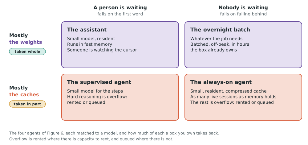
The dividing line is not light work against heavy work. It is what the agent does and who is waiting. Put a small model on the narrow, watched work, where the first word has to come quickly and code has already done the heavy lifting. The broad reasoning a small model fails at needs a big sparse one, and section 8 showed that one box serves it to one user at a time at best. So treat it as overflow, and bound its context, so the one expensive conversation does not crowd out twenty cheap ones. Give the always-on agents the smallest model and the leanest cache that keep pace, because for them the number of live sessions is the whole bill. Bound the thinking on the routine steps (section 7). And move everything with no deadline but the morning into the night. Belcak and others argue for the same split (section 8.8).
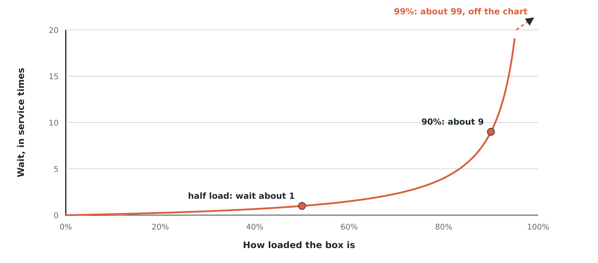
On owned hardware you cannot add capacity when demand spikes. Unless you rent the overflow, your only response is to make work wait, so what runs when is the decision the whole design rests on. Queues do not degrade gracefully. Time spent waiting in the queue rises as ρ/(1−ρ), where ρ is how loaded the box is: at half load a job waits about one service time before it starts, at 90 per cent about nine, at 99 per cent about ninety-nine. It hits a wall. So the daytime peak, the two kinds of agent with a person waiting, sizes the box, and the overnight batch runs in capacity that is already paid for. A business is not buying compute for the background work. It is using the twelve hours a day it already owns. Figure 19 shows the curve.
The queue is also the published cure for the collapse in section 3. Capping how many agents were live at once took that node from 0.6 requests a second back to about 2.25 (He, preprint, November 2026; measured). A peer-reviewed system gets the same effect by pausing whole agent programs (ThunderAgent, ICML 2026). All of that is on data-centre nodes. That the same lever holds on a business box is my reasoning. So is the next step: group the work by task, and some of the expert locality a mixed batch destroys should come back (section 5).
What the box cannot take is overflow, and there are two things to do with it. Where there is capacity to rent, and the data is allowed to leave the building, rent it: own the base, rent the peak (section 14). Where there is not, the work waits in the queue. Renting is the shared box again, with its wall and its grid queue, so the design treats it as the exception.
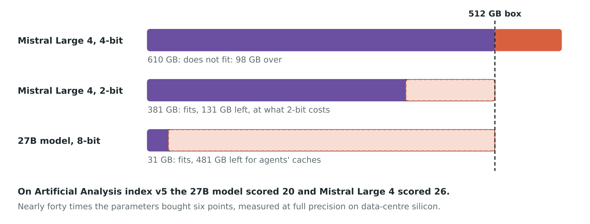
Do that and one fixed box does far more than its size suggests. Say it with its boundary, though. A 512 GB box with a 31 GB model resident has about 481 GB left for caches (Figure 20). At section 4’s figure for a small model, 4.3 GB for a conversation of 32,000 tokens, that is about 110 live sessions. A thousand fit only if each holds under about 3,700 tokens. An 8-bit cache would roughly double both, at the cost in section 8.7. That is my arithmetic on section 4’s table. Section 2 said a business on always-on agents runs thousands at once, and nobody has published how many a real one needs live. So the always-on row is a bet: short contexts, and the rest waits or is rented.
This is the design for a business running its own agents on its own work. It is not a design for serving the public at scale, and section 14 says so.
Worked example: the frontier model on your box against a model built for the job
Take the biggest open model you could plausibly put on a box, and put it on one. Mistral released the open weights of Mistral Large 4, nicknamed Le Chonk, on 29 October 2026: a mixture of experts with 1.05 trillion parameters, 52 billion of them active for each token. Mistral’s own 4-bit release is 610 GB and the common community build is 635 GB, before a single conversation’s cache. It does not fit a 512 GB box at 4-bit. To get it onto the largest unified-memory machine you can buy you have to go to 2-bit, at 381 GB or 298 GB, and section 8.2 says what that costs.
Now set against it a model built for the job: a 27B model at 8-bit, about 31 GB, resident in full, with room on a 512 GB box for a great many conversations’ caches. On version 5 of the Artificial Analysis index in November 2026 it scored 20, against Le Chonk’s 26, 46 for Kimi K3.1 Pro (the best model whose weights could be downloaded, at 1.56 TB, and scored through its maker’s API) and 59 for the closed frontier. On an open benchmark the big models win without trying. But look at the size of the first gap: nearly forty times the parameters bought six points, measured at full precision on data-centre silicon. Figure 20 shows what fits.
But the benchmark is the wrong comparison, and the way it is wrong is the point of this paper. Vendor benchmarks are run at full precision on data-centre silicon. Nobody is going to run Le Chonk at full precision in a server room. The fair comparison is the one nobody publishes: the frontier model quantised until it fits your box, with however many agents’ caches your box has left over, against a model built for the job, on the job. Not on a benchmark. On the invoices, the orders and the tickets your agents actually read.
What quantisation costs first is structured output and some multi-step tasks, the joint an agent depends on (ACBench, section 8.2). That cuts at the squeezed big model and at the small one too, so the test has to check the joint and not only the answer.
My claim, and it is a claim rather than a measurement until I run it, is that on narrow work with code doing the heavy lifting the small model matches the result, holds many conversations where the big one holds few, and answers before the person has looked away. That is a bet. If I am wrong about it, section 14 says what it does to the argument.
What this does not claim, and what would kill it
This paper does not claim four things, and it is worth being exact about them, because each is the strong version somebody will try to put in my mouth.
It does not claim that the wall binds a provider serving many users on big silicon, or that the box is the efficient choice. Batching works for them, soonest for dense models, and per answer a batched data centre beats the box (section 5). The box wins where the data centre cannot be had.
It does not claim that cloud is dearer to start. It usually is not. The people who sell the hardware will tell you cloud is cheaper to begin with, and they are right.
It does not claim that smaller is cheaper per token. It is not. High utilisation is what makes amortised silicon cheap per token, and a hyperscaler’s utilisation is one no single business will match. Yuan and Long work it through for one model: about $21 per million tokens on a single eight-GPU node against $0.26 on a 96-GPU cluster, roughly eighty times (analytical, by authors who sell a rival chip). Smaller decides who is allowed to own the thing at all. What a box can claim is the base load. One stylised model sends high-mean demand to private hosting and variable demand to the public cloud (Jain and Hazra, 2019, peer-reviewed; read in abstract). Applying it to always-on agents is my reasoning: own the base, rent the peak.
The strongest version of that objection came from the person best placed to make it. On 29 October 2026 Sam Altman said it was “quite terrible to have everybody have a bunch of the world’s limited supply of DRAM sitting in their own computer” and “being used… 5% of the time”, and that the answer was “maximum utilization in the cloud” (Cheeky Pint, episode 39, official transcript). He gave no source for the five per cent. My reading, and it is mine, is that even the buyer with the deepest pockets is short of memory and says so. For memory that sits idle he is right, and I concede it. But his five per cent is a picture of the first kind of agent: a person asks, reads, and the box waits. A box sized for the daytime peak and filled with the night’s work is not idle memory. It is memory a business already owns, in use around the clock, on data that never leaves the building.
And it does not claim frontier capability. It claims the job.
Five things would kill it, and I would rather name them than wait for them.
If offloading holds high expert-cache hit rates at large batch on a frontier mixture of experts, section 8.3 is wrong and the second-agent boundary was an engineering gap after all. I have found no such result; the nearest paper, which I have seen only in extract, points the other way.
If capacity arrives at bandwidth that keeps pace with demand, at a price one business can pay, so that a shared box holds thousands of conversations at speed without hundreds of GPUs, the shared-box track collapses. The earlier version of this test was met in March 2025 and strengthened the small box. The new one is the ratio in section 6.
If a small model on narrow work, with code doing the heavy lifting, does not match the result, act three falls. That is the bet in section 13, and I have not run it. Acts one and two would stand: the memory bill is real and the eight methods break where they break. But the box would hold the agents and fail the job, and the only answer left would be the industry’s.
If cheap, high-endurance storage makes a per-agent cache on the drive free of wear, the second half of section 8.4 falls and the small box gains a tier it does not have today. That one is moving. It is not met.
If decoding stops being bound by memory, the diagnosis itself moves. Two lines of work push that way: block-diffusion decoding, which one peer-reviewed paper measured shifting decode towards compute (FOCUS, ICML 2026), and speculative decoding (MagicDec, ICLR 2025). Both still keep a cache for every conversation, and I have found neither deployed at scale in a form that shrinks it. This one is open, and not triggered.
And the reverse case. If small models close the gap on broad reasoning, the paper gets stronger, not weaker, and I will say so when it happens.
One guard against myself, stated so you can hold me to it. Every absolute figure in this paper will date, and some will date fast: 24 tokens a second, 44 GB a wafer, the price of a box. Bigger memory moves the figures. It leaves the ratios standing: the weights are shared and the caches are not; the cache grows with every agent; the fetch costs more than the maths. Argue with the ratios. If the ratios fall, so does the paper.
What comes next
Why does everyone need so many data centres? Because agents in production are a memory problem, and the industry’s answer to a memory problem is to buy the memory. It has bought it in GPUs by the hundred, in wafers, in buildings by the gigawatt, and in 2026 it was buying it faster than the memory makers could make it, which is why memory cost more in 2026 than in 2025, all the way down to the laptop in your bag.
And if Europe wants its AI on its own soil, what does it do instead? It stops trying to out-buy the people with the deepest pockets in the history of computing, and it changes the question. Not how do we get more memory, but how much work can we get done on the memory we have. A model sized to the job, the whole of it resident. The domain as the unit of reuse. Each agent holding only what it needs. The night’s work run in the night. The data never leaving the building. None of that needs a place in the queue for a grid connection, and none of it needs a frontier model. It needs the result, and the result was always what the business was paying for.
Thesis 1 said the model was never meant to be the system. Thesis 2 said that where the work runs fixes what it costs. This paper has said what it costs to hold the model at all, and found that the answer decides who gets to own one. That leaves a question I have not touched here, and it is not a question about memory. A business that wants to run any of this has to put it into an operation built around a different worker. What that costs, every day it stays, is the next paper.
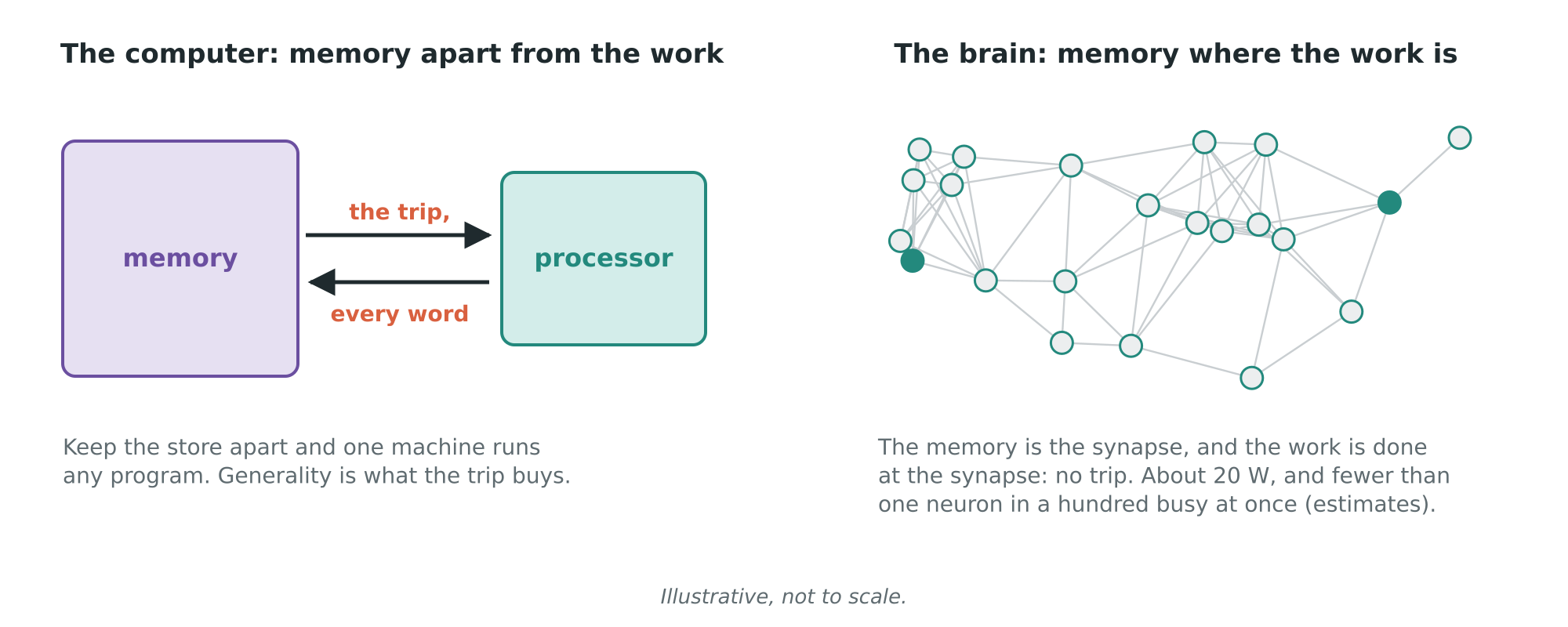
The brain does its work on about 20 W. That is the usual estimate, and nobody has put a meter on it. It has some 86 billion neurons, and on that budget fewer than one in a hundred can be busy at once (Lennie, 2003, an estimate). What it does not have is a trip (Figure 21). The memory is the synapse and the work is done at the synapse. Backus named the computer’s version of the trip in 1978, the von Neumann bottleneck, and the reason for it is a good one: keep the store apart from the processor and one machine can run any program. Generality is what the trip buys. Chips built the other way exist as research, IBM’s NorthPole among them, and I have found none shipped at scale. A sparse model copies half the trick: it fires few of its experts for each word, and still keeps every one of them in memory. Claim the job, not the model, and you are no longer paying for generality you do not use. So the last question is not how to make the trip shorter. Maybe we always moved the wrong part?
References
One entry per figure in the text, by section: what it supports, source, date, and how the figure was got (measured, derived, a rating, a position, or my reasoning). The twenty-one diagrams draw only on these sources; where a diagram adds arithmetic of its own, its caption says so. Full links, access dates and archive copies are available on request.
Opening
- five IBM System/360 Model 75 computers at Houston · Johnstone, AFIPS Spring Joint Computer Conference, 1969; IBM System/360 System Summary (A22-6810-0), 1964 · primary, confirmed. No speed, power or size figure is on a primary and none is used.
- bit flips between neighbouring memory rows (errors in 110 of 129 modules) · Kim et al., ISCA, June 2014 · measured by the source; read in extract only.
- about 5 GW of data centres connected by 2030 (5.2 GW) · NESO written evidence DCU0081 to the Environmental Audit Committee, from Future Energy Scenarios 2025 · 21 May 2026 · the operator’s forecast; primary; snapshot.
- a queue of about 73 GW (72.8 GW through to 2039) · Ofgem “Curate” consultation, 29 July 2026; NESO DCU0081, 21 May 2026 · primary; snapshot.
- perhaps half the queue speculative (“close to 50%” speculative or duplicate) · NESO Electricity Markets Advisory Council slides · 22 September 2026 · secondary until the slides are fetched.
- the wall from hardware trends · Gholami et al., “AI and Memory Wall”, IEEE Micro 44(3) · May to June 2024 · peer-reviewed; a fitted trend.
- the wall derived for data-centre GPUs · Singh (Dell), “The KV Cache Is the New Memory Wall” · September 2026 · preprint; derived; the author works for a hardware vendor.
- the wall from chip economics · Yuan and Long, “The Economics of AI Decoding Chips” · July 2026 · preprint; analytical; interested (they sell the chip they model).
Section 1 · Thesis
- more than one agent at once, measured on data-centre GPUs and on an Apple M4 Pro · Yuan et al. v2, September 2026; Shkolnikov, February 2026 · measured; preprints. Figures in section 4.
- “Europe cannot win that race” · Calderaro et al., European Security · 2022 · peer-reviewed; a position, not data; read in abstract only.
- the brain at about 20 W · Raichle and Gusnard, PNAS, 2002; Levy and Calvert, PNAS, 2021 · the usual estimate; no measurement was found.
- 100 W, the USB-C limit before 2021 · USB Promoter Group and USB-IF · May 2021 · a specification.
- 94 W and 138 W, a Mac Studio M3 Ultra while writing · Towards Data Science, the author’s own TokenWatt tool · July 2026 · one author’s measurement (chip counters checked against a wall meter); secondary; interested; not peer-reviewed.
- 2,990 W from one British socket · Electricity Safety, Quality and Continuity Regulations 2002, reg. 27; BS 1363 · 2002 · arithmetic on ratings (13 A at 230 V).
- about 120,000 W for one GB200 rack; forty sockets · NVIDIA DGX GB200 User Guide · undated, read 9 November 2026 · the maker’s rating; the forty is my arithmetic.
- about 5 billion W connected by 2030 · as the opening.
- Thesis 1 and Thesis 2 · thkdigital.com · own site.
Section 2 · Four kinds of agent
- two to two and a half turns; about 600 and 1,900 tokens a conversation · LMSYS-Chat-1M and WildChat, both ICLR 2024 · measured by the sources; the totals are my arithmetic from their means (568 and 1,872).
- 4,265 sessions from 43 developers; about 119,000 tokens re-read to write about 214 · TraceLab (Zhu et al.) · 30 June 2026 · measured; preprint; coding agents.
- cache-hit ratios 84.6 to 99.5 per cent; writing 91.0 to 98.6 per cent of model time; contexts 69,000 to 80,000 tokens · Yuan et al., “Agentic AI Workload Characterization” · May 2026 (v2 September 2026) · measured; preprint; coding benchmarks.
- no public trace of a business agent; the nearest production logs · arXiv 2608.15127 · August 2026 · gap confirmed; preprint seen in extract only.
- Concur, the nearest study of offline agent batches · arXiv 2601.22705 · January 2026 · preprint; abstract only (no figure taken).
- prompt length up about fourfold, around 1,500 to over 6,000 tokens · OpenRouter and a16z, “State of AI” · 4 December 2025 · measured on one platform.
- 76 to 80 per cent of the platform’s tokens from agents · OpenRouter’s October recap (6 November 2026, secondary); Menlo Ventures, “2026: The State of Enterprise AI” (3 November 2026, primary, on OpenRouter’s data) · one platform; tokens, not users.
- input cut by 39.9 to 59.7 per cent with the same results · AgentDiet (Xiao, Gao, Peng, Xiong), FSE · 2026 · measured; peer-reviewed; one coding agent, two models, two benchmarks; the results tables were not read.
Section 3 · Reactive means two things
- throughput from about 2.4 to about 0.6 requests a second as agents went from 20 to 32 · He (Huawei), arXiv 2611.01404 · 1 November 2026 · measured; preprint; four H800 GPUs, robot-control agents.
- the queueing condition and the job-size effect · Yang, Xu and Jiao, arXiv 2407.05347, 2024; Kingman, 1961 · mechanism only; no figure taken. The business job-size mix is reasoning.
Section 4 · What agents hold
- 327,680 bytes a token; crossovers at 427.2k tokens (one conversation) and 13.4k (32) · Singh, Table 4 · September 2026 · derived; preprint.
- 20 to 38 per cent of KV memory used before paging (20.4 to 38.2) · Kwon et al. (the vLLM paper) · September 2023 · measured by the source.
- the table: bytes per token, sizes at 32K and 128K, weights, crossovers of about 4, 13 and 290 · published model configurations; DeepSeek’s ISCA 2025 paper for 70,272 bytes · checked 3 November 2026 · my arithmetic on primary configurations.
- 7.5 GiB of weights against 9 GiB of cache at 16K and four conversations (Qwen3-4B) · KVSwap (Zhang, Xia, Wang) · November 2025 · a computed footprint; preprint.
- 52.56 billion of 54.90 billion input tokens cached; 186.9 million written · TraceLab, Table 1 · June 2026 · measured; preprint.
- 107 to 242 millijoules a token between 4K and 16K of context · Ma et al., arXiv 2605.11999 v1 (accepted by PPAM 2026) · 2026 · sensor (the GPU alone); about 4B models on one H200; a v1 figure not checked against v2.
- cache-hit rate 98.85 to 16.78 per cent and 30.08 to 16.96 tokens a second per request, 15 to 20 agents · Yuan et al. v2, Table II (Qwen3.6-27B, two H100 NVL) · 21 September 2026 · measured; preprint.
- re-reading stretches a request by up to 7.14 times · ThunderAgent, ICML 2026 · measured; peer-reviewed; one 8×H100 node; an inference vendor among the authors.
- 10.2 GB of cache budget; six agents at 4K, three at 8K; 15.7 s to re-read against 577 ms to restore from disk (Gemma 3 12B) · Shkolnikov, “Agent Memory Below the Prompt” · 17 February 2026 · measured; single-author preprint.
Section 5 · The fetch
- the measure: speed is bandwidth over bytes read per word; energy is bytes times cost per byte, plus standing power · my definition · 9 November 2026 · a definition. The bytes read are the active weights plus the conversation’s cache.
- decode is memory-bound by construction · Singh · September 2026 · derived; preprint.
- 140 GB at 3.35 TB/s is about 24 tokens a second (23.9) · NVIDIA H100 SXM specification · read July 2026 · arithmetic on the maker’s figures.
- 0.270 of the bandwidth floor on an H100, 0.810 on an L4 (Qwen-2.5-7B) · Chen, “Memory-Bound but Not Bandwidth-Limited”, Table 1 · May 2026 · measured; preprint; 7B scale. Beyond 7B it is reasoning.
- operands from external DRAM cost about 200 times the arithmetic (more than 10 nJ against about 50 pJ) · Keckler, Dally, Khailany, Garland and Glasco, IEEE Micro 31(5) · September 2011 · the source’s figures for 40 nm hardware; NVIDIA authors.
- 3.4 to 4.5 picojoules a bit: HBM3E 3.44 (SK hynix, IEDM 2023, implied), LPDDR5X 4 (Micron), GDDR7 4.5 (Micron) · 2023 and undated maker documents · the makers’ own figures; different boundaries; none measured by a third party; the LPDDR5X figure seen in a snippet only.
- an SSD at thirty to nearly fifty times that (125 to 161 picojoules a bit) · Micron 9550 datasheet · undated · arithmetic on a rating.
- the energy goes into charging the wire; high speeds force short wires · Keckler et al. 2011 for the capacitance mechanism · 2011 · mechanism.
- 138 W at 21.5 tokens a second (Qwen3.6-27B, dense, 8-bit) and 94 W at 74 (gpt-oss-120b, about 5B active) · Towards Data Science, TokenWatt · July 2026 · one author’s measurement; secondary; interested; not peer-reviewed.
- a fraction of a penny an answer (0.1764 Wh at 24.51p per kWh is 0.0043p) · DESNZ Quarterly Energy Prices, September 2026 · my arithmetic.
- the ridge near 295 on an H100 (989 TFLOPS over 3.35 TB/s) · Singh; NVIDIA specification · 2026 · derived.
- 0.15 to 0.31 joules a token (Qwen 3 32B on one B200, batch 128 to 512) · Chung et al., arXiv 2601.22076 v1, Table 1 · 29 January 2026 · sensor (the GPU alone); preprint.
- 6.4 joules a token on the desk (138 W over 21.5 tokens a second) · as the Mac Studio run · arithmetic on one run.
- attention stays memory-bound as the batch grows · Recasens et al., IEEE CLOUD 2025 · measured (OPT-1.3B on an H100); peer-reviewed.
- a “MoE tax” of 32 times; about 4,700 users per H100 for DeepSeek-R1 · Yuan and Long, §3 · July 2026 · derived; preprint; interested.
Section 6 · How memory was moved closer
- efficiency doubled every 1.57 years, 1946 to 2009; later every 2.6 years; a hundredfold a decade against sixteenfold · Koomey et al., IEEE Annals of the History of Computing 33(3), 2011; Koomey and Naffziger, 2015 and 2016 · the authors’ historical trend (captions and abstract read) and their own later statements.
- Dennard’s rule and its end in leakage · Dennard et al., IEEE JSSC, October 1974 (reprint excerpt); Horowitz, ISSCC, February 2014 · primary; mechanism.
- logic gained more than wires · Keckler et al., IEEE Micro, 2011 · the source’s statement; NVIDIA authors.
- “memory wall” named · Wulf and McKee, ACM SIGARCH Computer Architecture News 23(1) · March 1995 · primary.
- compute 3.0 times every two years against memory bandwidth 1.6 and interconnect 1.4, over twenty years · Gholami et al., IEEE Micro 44(3) · 2024 · peer-reviewed; fitted trends.
- H100: 80 GB at 3.35 TB/s · NVIDIA specification · read July 2026 · the maker’s specification.
- Cerebras WSE-3: 44 GB of SRAM on one wafer; about 6,400 to one on bandwidth (21.6 PB/s) · Cerebras · August 2026 · the maker’s own figures; the ratio is my arithmetic (6,448).
- no catalogue model fitted one wafer at 16-bit · Cerebras public catalogue · October 2026 · snapshot; arithmetic on the maker’s catalogue.
- stacked memory up 1.35 times a GB, 2023 to 2025; DDR4 down to 0.54 times, 2022 to 2025 · Ma and Patterson, IEEE Computer, Fig. 3 · February 2026 · the source’s figures; Google authors; the two windows differ.
- Rubin at 19.2 TB/s per GPU against up to 22 in earlier announcements · NVIDIA specification pages and developer blog · read 9 November 2026 · the maker’s specification; snapshot.
- Mac Studio: up to 512 GB at 819 GB/s (M3 Ultra, 5 March 2025) and 1.2 TB/s (M5 Ultra, 25 August 2026) · Apple · the maker’s specification.
- 512 GB withdrawn in March 2026; back on 28 October 2026 on the M5 Ultra; the option $15,500 against $4,000 · Cult of Mac, 9to5Mac, MacRumors · March and October 2026 · secondary; Apple’s store page was not captured.
- the ratio: bandwidth 1.6 times every two years against prompt length up about fourfold in a year · Gholami et al.; OpenRouter and a16z · the ratio itself is unpriced.
- a 27B model at 8-bit is about 31 GB (Qwen3.8 27B, 30.9 GB) · Hugging Face file sizes · 3 November 2026 · snapshot.
Section 7 · The wait before the first word
- about five or six tokens a second (238 words a minute) · Brysbaert, Journal of Memory and Language 109 · 2019 · a meta-analysis; the token rate is my arithmetic.
- streaming at 14 to 1,638 tokens a second; first chunk at maximum effort 253 to 641 seconds · Artificial Analysis · 3 November 2026 · a third party’s measurements through the makers’ APIs; snapshot.
- the early scheduling agent often took about three minutes; users gave up after about one · my own account · own data; one build.
- 240 participants; waits of 2, 9 and 20 seconds; impatience beginning at 20; nothing tested beyond · Tan, Messerschmidt, Yin and Nov, CHI 2026 · measured; peer-reviewed. The absence of a longer test is a confirmed gap.
- the shortest of twenty answers beat the longest by up to 34.5 percentage points (one model’s maths average) · Hassid, Synnaeve, Adi and Schwartz · February 2026 · measured; preprint; the table was read in extract.
- the bet’s footing: most tokens on one platform; a longer session is a bigger cache · as sections 2 and 4.
- conventional DRAM contract prices up about 93 to 98 per cent in the first quarter of 2026 · TrendForce · 1 June 2026 · an analyst’s outturn figure.
- “effectively sold out” through 2029; contracts covering more than half of 2027 and 2028 capacity · SK hynix third-quarter call and release · 28 October 2026 · the call is an interpreted transcript (secondary; the speaker is not settled); the release is primary.
Section 8 · Eight methods
- 8.1 and 8.6: 671B total, 37B active; 320 GPUs in 40 nodes specified, 144 in 18 in production · DeepSeek technical report, 27 December 2024; infrastructure note, 1 March 2025 · the maker’s own figures.
- 8.1: $1.20 per million output tokens at peak · DeepSeek pricing · read 3 November 2026 · the maker’s price; snapshot; last re-read from a secondary.
- 8.1: 763B stored, 16B active per written token (V4.1 Flash) · the model card · October 2026 · the maker’s own figures.
- 8.1: about 0.6 per cent of the arithmetic used on an eight-GPU node · Yuan and Long, §3 · July 2026 · derived; interested.
- 8.1: 70 KB against 516 KB a token; 86.4 per cent smaller · DeepSeek, ISCA 2025, Table 1 · May 2025 · the maker’s figures; the percentage is my arithmetic.
- 8.2: 720 GB to 131 GB; 69.2 against 91.7 per cent; attention at 4 or 6 bits · Unsloth · 27 January 2025 · a vendor’s demonstration on its own test.
- 8.2: 8-bit lossless over 500,000 evaluations; up to 59 per cent lost at long context at 4-bit; more than 7 per cent at 3-bit · Kurtic et al., ACL 2025; Mekala et al., EMNLP 2025; Liu et al., COLM 2025 · measured; peer-reviewed; Kurtic’s authors sell quantised models.
- 8.2: about half a point to four points at 4-bit; tool use down 0.4 to 3.6 points at 7B; structured output degrades more · Kurtic et al., ACL 2025; ACBench, ICML 2025 · measured; peer-reviewed; read in full. The guard (constrained decoding and validation) is my addition.
- 8.3: 14 GB of GPU memory plus 382 GB of RAM; 8.73 to 13.69 tokens a second · KTransformers · February 2025 · the project’s own figures.
- 8.3: latency scales with the experts activated across the batch · Lynx, arXiv 2411.08982 · November 2024 · preprint; abstract only (no figure taken).
- 8.3: hit rate 76.61 to 58.37 per cent, batch 4 to 16 · ExpertFlow (He et al.), DAC 2026 · measured; peer-reviewed; a small model (Switch-32) only.
- 8.3: up to 10.3 times the throughput; 30.12 tokens a second across 504 sequences · MoE-Lightning, ASPLOS 2025 · measured; peer-reviewed; Mixtral 8x7B on one 16 GB GPU; offline batch only.
- 8.4: GPU memory at 2 to 3.35 TB/s; a fast NVMe drive at about 14 GB/s · NVIDIA and Samsung specifications · ratings.
- 8.4: a 744B model at 0.05 to 0.1 tokens a second on a laptop · Colibri README v2.1.0 · read 3 November 2026 · the project’s own figures.
- 8.4: a 35 GB model streamed whole: 2.4 to 4.7 seconds a word; 19.29 to 27.25 joules a word for the drive alone · Samsung 990 PRO and 9100 PRO datasheets · arithmetic on ratings, labelled as such.
- 8.4: streamed expert weights at roughly 4 to 12 times the energy per token of stacked memory · Kyung, Yun and Ahn, IEEE Computer Architecture Letters 24(2) · 2025 · simulated; peer-reviewed; part-funded by Samsung.
- 8.4: 8.6 TB a day; thirteen times a 2 TB consumer drive’s daily budget; warranty gone in about 140 days · Samsung 990 Pro endurance · my arithmetic; the write pattern is an assumption.
- 8.4: 0.2 to 0.4 years of drive life at data-centre scale; no drive-measured wear anywhere · Gandalf · 22 October 2026 · computed from trace write volume against rated endurance; preprint; a storage maker among the authors. The gap is confirmed.
- 8.4: flash ruled out for a cache updated at every token · Ma and Patterson, IEEE Computer · February 2026 · the authors’ argument; Google authors.
- 8.5: the ridge near 295; a sparse model stays memory-bound · as section 5.
- 8.6: 44 GB a wafer · as section 6.
- 8.6: 2.3 times less energy; 5.2 times the tokens per dollar · CENT, ASPLOS 2025 (the published abstract) · simulated; peer-reviewed.
- 8.6: Samsung’s processing-in-memory found only in test systems · Samsung technical blog; Hot Chips 2023 · the maker’s own account; other products were not searched.
- 8.6: a 512 GB, 819 GB/s card at about $19,000 built · Yuan and Long, §6 · July 2026 · the authors’ own estimate; interested.
- 8.7: V4-Pro needs a tenth of V3.2’s cache at a million tokens · DeepSeek’s own report · April 2026 · the maker’s own figure.
- 8.7: 1.25 times at one conversation, 4.82 times at a batch of 32 (2-bit cache, Llama 3 70B, B200, 128k) · Singh, Table 7 · 25 September 2026 · derived bounds; preprint.
- 8.7: five to ten points lost on RULER-128K with an 8-bit cache (gpt-oss-120B) · NVIDIA Puzzle technical report, Table 2 · 12 February 2026 · the maker’s own evaluation.
- 8.8: 224 of 310 fine-tuned models beat GPT-4 · LoRA Land (Zhao et al.) · April 2024 · measured; preprint.
- 8.8: 1.3 points on Spider · OmniSQL-7B (Li et al.) · March 2025 · measured; preprint.
- 8.8 and 12: 40 to 70 per cent of calls in three agent systems could go to small models · Belcak et al. (NVIDIA) · 2025, v3 September 2026 · a position paper; estimates; no experiment.
- 8.8: GPT-4 beat BloombergGPT and Med-PaLM 2 · Li et al., EMNLP 2023; Nori et al., November 2023 · measured.
- 8.8: 44 GB scores 20, 128 GB scores 28 (2-bit), 512 GB scores 32 · Artificial Analysis Index v5 and Hugging Face file sizes · 3 November 2026 · snapshot.
Section 9 · The same place
- No new figures. The table and Figure 12 restate section 8’s verdicts.
Section 10 · The shared data centre
- about 5 GW connected by 2030 on the ten-year forecast · NESO written evidence DCU0081 · 21 May 2026 · the operator’s forecast; primary.
- a queue of about 73 GW · Ofgem “Curate” consultation · 29 July 2026 · primary.
- close to half the queue speculative or duplicate · NESO Electricity Markets Advisory Council slides · 22 September 2026 · secondary until fetched.
- about 40 per cent of identified capacity at a final investment decision (20 of 50 GW) · Ofgem Demand Connections Call for Input · 13 February 2026 · primary; the percentage is by capacity.
- OpenAI paused its UK build; the quoted statement · emailed statement as carried by Bloomberg, Reuters and the BBC · 9 April 2026 · confirmed wording; secondary carriers.
- Texas paused large-load studies with about 474 GW queued · ERCOT Senate testimony, 29 July 2026; market notice, 3 August 2026; board slides, 11 September 2026 · primary.
- 138 W on a socket rated for 2,990 W · as sections 1 and 5.
Section 11 · One principle
- making and buying AI often done together, 3,143 European firms · Hoffreumon et al., Journal of Economics and Management Strategy · 2024 · peer-reviewed; a cross-section; read in abstract only. No study pricing sovereignty or lock-in was found.
Section 12 · Route each agent
- waiting of about one, nine and ninety-nine service times at 50, 90 and 99 per cent load, as ρ/(1−ρ) · standard queueing theory · arithmetic.
- an admission cap takes the node from 0.6 back to about 2.25 requests a second · He, arXiv 2611.01404 · 1 November 2026 · measured; preprint.
- pausing whole agent programs · ThunderAgent, ICML 2026 · peer-reviewed. On a business box the queue lever is reasoning.
- the pointers to sections 7 and 8.8 · as those sections.
Section 13 · Worked example
- Mistral Large 4: weights released 29 October 2026; 1.05T parameters, 52B active with embeddings; 610 GB (Mistral’s 4-bit) and 635 GB (community); 381 GB or 298 GB at 2-bit; 26 on the index · Mistral model documentation and Hugging Face files · October 2026 · the maker’s figures and file sizes.
- the 27B model: about 31 GB at 8-bit; 20 on Index v5; 59 for the best closed model · Artificial Analysis; Hugging Face · 3 November 2026 · snapshot.
- Kimi K3.1 Pro: 46 on Index v5.0.1, measured through the maker’s API; 1,561 GB of weights released 4 November 2026 · Artificial Analysis; Moonshot · November 2026 · snapshot; the score is not from the released weights.
- “nearly forty times the parameters bought six points” · arithmetic on the rows above (1.05T over 27B; 26 less 20).
- the named risk · ACBench, ICML 2025 · as section 8.2.
- the comparison itself · not yet run · a bet.
Section 14 · Does not claim, would kill
- about $21 against $0.26 per million tokens, roughly eighty times · Yuan and Long, §4 · July 2026 · analytical; interested.
- high-mean demand hosted privately, variable demand to the public cloud · Jain and Hazra, Production and Operations Management 28(5) · 2019 · peer-reviewed; a stylised model; abstract only. Applying it to agents is reasoning.
- the DRAM passage · Sam Altman, Cheeky Pint episode 39, official transcript · 29 October 2026 · primary; quoted from the canonical text. The five per cent has no source.
- first kill condition not triggered; the nearest paper points the other way · Diff-MoE, SC 2025 · seen in extract only; model scale not verified.
- the earlier test met in March 2025 · as section 6.
- fifth kill condition: block-diffusion and speculative decoding; neither found deployed in a form that shrinks the cache · FOCUS, ICML 2026; MagicDec, ICLR 2025 · measured; peer-reviewed; the gap is confirmed.
Section 15 · What comes next
- memory cost more in 2026 than in 2025 · TrendForce · June 2026 · as section 7.
- about 20 W; some 86 billion neurons; fewer than one in a hundred active at once · Levy and Calvert, 2021 (the 20 W as a convention); Azevedo et al., 2009; Lennie, Current Biology, 2003 · the 20 W is the usual estimate, not a measurement; Lennie’s figure is an estimate.
- the von Neumann bottleneck · Backus, Communications of the ACM 21(8) · August 1978 · primary.
- chips built the other way exist as research; none found shipped at scale · Modha et al. (IBM), Science, October 2023; Samsung · the makers’ own accounts; no figure taken.